% Changing Chebfun's operator preferences
cheboppref('maxdegree',10000)   % changing maximum degree of functions
cheboppref('restol',1e-6)       % changing residual tolerance

% System parameters
kx = 1; % streamwise wavenumber
kx2 = kx*kx; kx4 = kx2*kx2;

om = 0; % temporal frequency

beta = 0.5; % viscosity ratio

Weval = [1, linspace(10,100,10)]; % Weissenberg numbers
Wegrd = length(Weval);

dom = domain(-1,1);     % domain of your function
y = chebfun('y',dom);
fone = chebfun(1,dom);      % one function
fzero = chebfun(0,dom);     % zero function

% Boundary conditions
Wa0{1} = [1, 0, 0, 0; 0, 1, 0, 0];
Wb0{1} = [1, 0, 0, 0; 0, 1, 0, 0];

% Looping over Weissenberg number
Smax = zeros(Wegrd,1); A0 = cell(1,1); B0 = cell(1,2); C0 = cell(2,1);

for indWe = 1:Wegrd

    We = Weval(indWe);

    % coefficients of the operators A0 and B0
    a0 = (kx4*(1 + 1i*om + 1i*kx*We*y).*(beta - ...
        (2*(-1 + beta)*We*We*(1 + 2*We*We))./((1 + 1i*om + ...
        1i*kx*We*y).^3) - ((-1 + beta)*(1 + 2*We*We))./(1 + ...
        1i*om + 1i*kx*We*y)))./(1 + beta*(1i*om + 1i*kx*We*y));

    a1 = (2*1i*(-1 + beta)*kx2*kx*We*(1i*om + ...
        1i*kx*We*y).*(1 + 1i*om - 2*We*We + ...
        1i*kx*We*y))./(((1 + 1i*om + 1i*kx*We*y).^2).*(1 + ...
        beta*(1i*om + 1i*kx*We*y)));

    a2 = (2*kx2*(-1 - (1i*om + 1i*kx*We*y).*(2 + 1i*om + ...
        1i*om*We*We + 1i*kx*(We + (We^3)).*y + ...
        beta*(1 + (1i*om + 1i*kx*We*y).*(2 + 1i*om - We*We + ...
        1i*kx*We*y)))))./(((1 + 1i*om + ...
        1i*kx*We*y).^2).*(1 + beta*(1i*om + 1i*kx*We*y)));

    a3 = (2*(-1 + beta)*kx*We*(-1i*1i*om + kx*We*y))./((1 + 1i*om + ...
        1i*kx*We*y).*(1 + beta*(1i*om + 1i*kx*We*y)));

    b1 = -((1 + 1i*om + 1i*kx*We*y))./(1 + beta*(1i*om + 1i*kx*We*y));

    b0 = 1i*kx*((1 + 1i*om + 1i*kx*We*y))./(1 + beta*(1i*om + ...
        1i*kx*We*y));

    % system operators
    % coefficients of the operators A0 and B0
    % a0*phi + a1*phi' + a2*phi'' + a3*phi''' + 1*phi'''' =
    % 0*d1 + b1*d1' + b0*d2 + 0*d2'

    A0 = {[a0, a1, a2, a3, fone]};

    B11 = [fzero, b1]; B12 = [b0, fzero];
    B0 = {B11, B12};

    % coefficients of the operator C0
    % u = phi'; v = -i*kx*phi
    C11 = [fzero, fone]; C21 = [-1i*kx*fone, fzero];
    C0 = {C11; C21};

    % determine principal singular pair of the frequency response operator
    [Sfun,Sval] = svdfr(A0,B0,C0,Wa0,Wb0,1,1);

    % storing the largest singular value for each Weissenberg number
    Smax(indWe) = Sval(1);

end

% Plotting the largest singular value as a function of Weissenberg number
plot(Weval,Smax,'x-','LineWidth',1.1,'MarkerSize',10);
xlab = xlabel('We', 'interpreter', 'tex');
set(xlab, 'FontName', 'cmmi10', 'FontSize', 20);
h = get(gcf,'CurrentAxes');
set(h,'FontName','cmr10','FontSize',15,'xscale','lin','yscale','lin');
Two-dimensional inertialess shear-driven channel flow of viscoelastic fluids
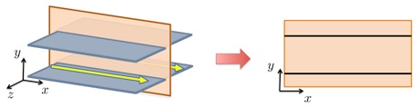 |
Two-dimensional channel flow geometry. |
We consider a system that describes the dynamics of two-dimensional velocity and polymer stress fluctuations in an inertialess shear-driven channel flow of viscoelastic fluids. The input-output differential equation representing the frequency response operator is given by
![begin{array}{l} left( D^{(4)} , + , a_{3}(y) , D^{(3)} , + , a_{2}(y) , D^{(2)} , + , a_{1}(y) , D^{(1)} , + , a_{0}(y) right) phi (y) [0.15cm] ; = ; b_{1}(y) , D^{(1)} , d_{1}(y) , + , b_{0}(y) , d_{2}(y), ;;; y , in , left[ -1, 1 right], end{array}](eqs/530330399927374942-130.png)
where
 | — | streamfunction |
 , ,  | — | streamwise and wall-normal forcing. |
The boundary conditions are given by

The desired outputs are the streamwise and wall-normal velocity fluctuations,
![begin{array}{rcl} u(k_x, y, t) & !! = !! & D^{(1)} , phi(k_x, y, t) [0.15cm] v(k_x, y, t) & !! = !! & -mathrm{i} , k_x , phi(k_x, y, t). end{array}](eqs/6403025569654224186-130.png)
Matlab codes
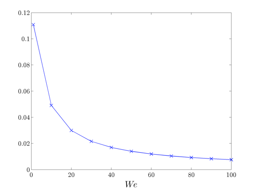
Determine the largest singular value of the frequency response operator, as a function of the
Weissenberg number  , for an inertialess shear-driven channel flow of viscoelastic fluids
with
, for an inertialess shear-driven channel flow of viscoelastic fluids
with  ,
,  , and
, and  .
.
 |
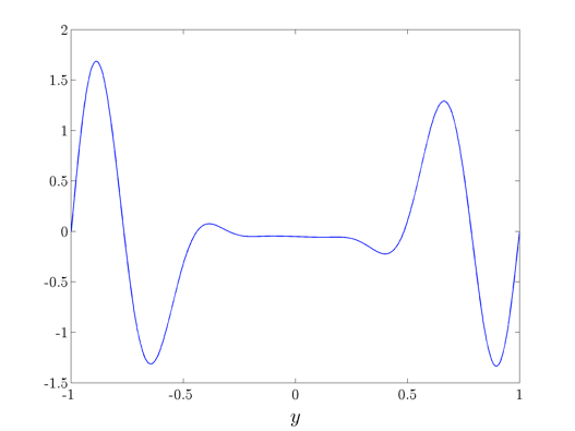
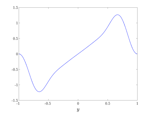
Plot the principal singular functions for  .
.
% principal singular function corresponding to the streamwise velocity
u = Sfun{1};
% principal singular function corresponding to the wall-normal velocity
v = Sfun{2};

% Plotting the most amplified streamwise velocity profile
plot(y,real(u)/norm(real(u)),'x-','LineWidth',1.1,'MarkerSize',10);
xlab = xlabel('y', 'interpreter', 'tex');
set(xlab, 'FontName', 'cmmi10', 'FontSize', 20);
h = get(gcf,'CurrentAxes');
set(h,'FontName','cmr10','FontSize',15,'xscale','lin','yscale','lin');
 |
% Plotting the most amplified wall-normal velocity profile
plot(y,real(v)/norm(real(v)),'x-','LineWidth',1.1,'MarkerSize',10);
xlab = xlabel('y', 'interpreter', 'tex');
set(xlab, 'FontName', 'cmmi10', 'FontSize', 20);
h = get(gcf,'CurrentAxes');
set(h,'FontName','cmr10','FontSize',15,'xscale','lin','yscale','lin');
 |