% System parameters:
R = 2000; % Reynolds number

kzval = linspace(0.1,5,30); % spanwise wave-number
kzgrd = length(kzval);

om = 0; % temporal frequency

dom = domain(-1,1);     % domain of your function
y = chebfun('y',dom);
fone = chebfun(1,dom);      % fone(y) = 1
fzero = chebfun(0,dom);     % fzero(y) = 0

U = diag(1 - y.^2);    % in pressure-driven flow
Uy = diag(-2*y);
Uyy = diag(-2*fone);

% Boundary conditions
Wa0{1} = [1, 0, 0, 0; 0, 1, 0, 0];
Wa0{2} = [1, 0];
Wb0{1} = [1, 0, 0, 0; 0, 1, 0, 0];
Wb0{2} = [1, 0];

% Looping over kz
Smax = zeros(kzgrd,1); A0 = cell(2,2); B0 = cell(2,3); C0 = cell(3,2);

for indz = 1:kzgrd

    kz = kzval(indz); kz2 = kz*kz; kz4 = kz2*kz2;

    % coefficients of the operator A0
    % kz^2*(kz^2/R + i*om)*phi1 + 0*phi1' - (2*kz^2*R + i*om)*phi1'' +
    % 0*phi1''' + (1/R)*phi1'''' + 0*phi2 + 0*phi2' + 0*phi2''
    A11 = [kz2*(kz2/R + 1i*om)*fone, fzero, ...
        -(2*kz2/R + 1i*om)*fone, fzero, (1/R)*fone];

    A12 = [fzero, fzero, fzero];

    % -i*kz*U?*phi1 + 0*phi1' + 0*phi1'' + 0*phi1''' + 0*phi1'''' -
    % (kz^2/R + i*om)*phi2 + 0*phi2' + (1/R)*phi2''
    A21 = [-1i*kz*Uy*fone, fzero, fzero, fzero, fzero];
    A22 = [-(kz2/R + 1i*om)*fone, fzero, (1/R)*fone];

    A0 = {A11, A12; A21, A22};

    % coefficients of the operator B0
    % 0*d1 + 0*d1' - i*kz*d2 + 0*d2' + 0*d3 + 1*d3'
    B11 = [fzero, fzero]; B12 = [-1i*kz*fone, fzero];
    B13 = [fzero, fone];

    % -1*d1 + 0*d1' + 0*d2 + 0*d2' + 0*d3 + 0*d3'
    B21 = [-fone, fzero]; B22 = [fzero, fzero]; B23 = [fzero, fzero];

    B0 = {B11, B12, B13; B21, B22, B23};

    % coefficients of the operator C0
    % u = 0*phi1 + 0*phi1' + 1*phi2 + 0*phi2'
    C11 = [fzero, fzero]; C12 = [fone, fzero];

    % v = i*kz*phi1 + 0*phi1' + 0*phi2 + 0*phi2'
    C21 = [1i*kz*fone, fzero]; C22 = [fzero, fzero];

    % w = 0*phi1 - 1*phi1' + 0*phi2 + 0*phi2'
    C31 = [fzero, -fone]; C32 = [fzero, fzero];

    C0 = {C11, C12; C21, C22; C31, C32};

    % solving for the left principal singular pair
    [Sfun, Sval] = svdfr(A0,B0,C0,Wa0,Wb0,1,1);

    % saving the largest singular value for each value of kz
    Smax(indz) = Sval(1);

end

% Plotting the largest singular value as a function of kz at a fixed om
plot(kzval,Smax,'-','LineWidth',1.1);
xlab = xlabel('k_z', 'interpreter', 'tex');
set(xlab, 'FontName', 'cmmi10', 'FontSize', 20);
h = get(gcf,'CurrentAxes');
set(h,'FontName','cmr10','FontSize',15,'xscale','lin','yscale','lin');
Streamwise-constant three-dimensional channel flow
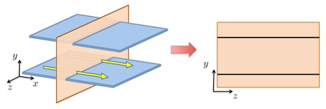 |
Streamwise-constant three-dimensional channel flow. |
Here, we consider the dynamics of the streamwise-constant fluctuations in three-dimensional channel flows,
![begin{array}{rcl} Delta , phi_{1, t} (k_z, y, t) & !! = !! & {displaystyle frac{1}{R}} Delta^{2} , phi_{1}(k_z, y, t) , + , mathrm{i} , k_z , d_{2}(k_z, y, t) , - , D^{(1)} , d_{3}(k_z, y, t) [0.4cm] phi_{2,t} (k_z, y, t) & !! = !! & {displaystyle frac{1}{R}} Delta , phi_{2}(k_z, y, t) , - , mathrm{i} , k_z , U'(y) , phi_{1}(k_z, y, t) , + , d_{1}(k_z, y, t) [0.4cm] y & !! in !! & left[ -1, 1 right] end{array}](eqs/1816983876775667000-130.png)
where
 , ,  | — | streamfunction and streamwise velocity |
 , ,  , ,  | — | streamwise, wall-normal, and spanwise forcing |
 | — | Reynolds number |
 | — | spanwise wavenumber |
 | — | for shear-driven flow |
 | — | for pressure-driven flow |
 | — | Laplacian |
 . . | ||
The boundary conditions are given by
![begin{array}{rcl} phi_{1}(k_x, pm 1, t) & !! = !! & D^{(1)} phi_{1}(k_x, pm 1, t) ; = ; 0 [0.15cm] phi_{2}(k_x, pm 1, t) & !! = !! & 0. end{array}](eqs/5224801892889218865-130.png)
The desired outputs are the streamwise, wall-normal, and spanwise velocity fluctuations,
![begin{array}{rcl} u(k_z, y, t) & !! = !! & phi_{2}(k_z, y, t) [0.15cm] v(k_z, y, t) & !! = !! & mathrm{i} , k_z , phi_{1}(k_z, y, t) [0.15cm] w(k_z, y, t) & !! = !! & -D^{(1)} , phi_{1}(k_z, y, t). [0.15cm] end{array}](eqs/8837882810514837915-130.png)
The input-output differential equations representing the frequency response operator are given by
![begin{array}{rcl} {displaystyle left( frac{1}{R} , D^{(4)} , - , left( frac{2 , k_z^2}{R} , + , mathrm{i} , omega right) D^{(2)} , + , k_z^2 left( frac{k_z^2}{R} , + , mathrm{i} , omega right) right) , phi_1 (y) } & !! = !! & - mathrm{i} , k_z , d_{2}(y) , + , D^{(1)} , d_{3}(y) [0.45cm] {displaystyle left( frac{1}{R} , D^{(2)} , - , left( frac{k_z^2}{R} + mathrm{i} , omega right) right) phi_2 (y) , - , mathrm{i} , k_z , U'(y) , phi_1 (y) } & !! = !! & - d_1 (y). end{array}](eqs/3754853323050110636-130.png)
Matlab codes
Determine the largest singular value of the frequency response operator for the streamwise-constant
pressure-driven channel flow with  as a function of . Since slowly-varying structures
exhibit largest amplification, we set the temporal frequency to zero,
as a function of . Since slowly-varying structures
exhibit largest amplification, we set the temporal frequency to zero,
 .
.
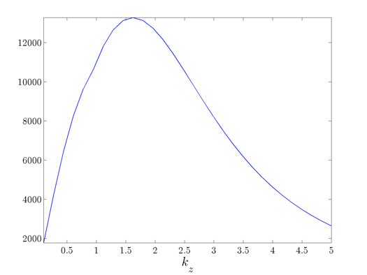 |
The spanwise wavenumber |
 at which the largest singular value peaks identifies the
length scale
at which the largest singular value peaks identifies the
length scale  of the most amplified velocity fluctuations.
 Determine the most amplified streamwise-constant flow structures in a pressure-driven
channel flow with , , and  .
.
% System parameters:
N = 100;    % number of collocation points for plotting
yd = chebpts(N);

kz = 1.62; kz2 = kz*kz; kz4 = kz2*kz2;
om = 0;

% coefficients of the operator A0
A11 = [kz2*(kz2/R + 1i*om)*fone, fzero, ...
    -(2*kz2/R + 1i*om)*fone, fzero, (1/R)*fone];
A12 = [fzero, fzero, fzero];
A21 = [-1i*kz*Uy*fone, fzero, fzero, fzero, fzero];
A22 = [-(kz2/R + 1i*om)*fone, fzero, (1/R)*fone];

A0 = {A11, A12; A21, A22};

% coefficients of the operator B0
B11 = [fzero, fzero]; B12 = [-1i*kz*fone, fzero]; B13 = [fzero, fone];
B21 = [-fone, fzero]; B22 = [fzero, fzero]; B23 = [fzero, fzero];
B0 = {B11, B12, B13; B21, B22, B23};

% coefficients of the operator C0
C11 = [fone, fzero]; C12 = [fzero, fzero];
C21 = [fzero, fzero]; C22 = [fone, fzero];
C0 = {C11, C12; C21, C22};

% solving for the left principal singular pair
[Sfun, Sval] = svdfr(A0,B0,C0,Wa0,Wb0,1,1);

% streamfunction and streamwise velocity
psii = Sfun{1}; % streamfunction
ui = Sfun{2}; % streamwise velocity

% discretized values for plotting
pvec(:,1) = psii(yd,1); uvec(:,1) = ui(yd,1);

% Getting physical fields of u and psi
zval = linspace(-2*pi/kz, 2*pi/kz, 100); % spanwise coordinate

Up = zeros(N,length(zval));   % physical value of u
Pp = zeros(N,length(zval));   % physical value of v

for indz = 1:length(zval)

    z = zval(indz);

    Up(:,indz) =  Up(:,indz) + ...
        uvec*exp(1i*kz*z) + conj(uvec)*exp(-1i*kz*z);

    Pp(:,indz) =  Pp(:,indz) + ...
        pvec*exp(1i*kz*z) + conj(pvec)*exp(-1i*kz*z);

end

Up = real(Up); Pp = real(Pp); % only real part exist

% Plotting the most amplified streamwise velocity structures (color plot)
pcolor(zval,yd,Up/max(max(Up))); shading interp;

% Plotting the most amplified streamfunction structures (contour plot)
Ppn = Pp/max(max(Pp));
hold on
contour(zval,yd,Ppn, ...
    linspace(0.1*max(max(Ppn)),0.9*max(max(Ppn)), 4),'k--','LineWidth',1.1)
contour(zval,yd,Ppn, ...
    linspace(-0.9*max(max(Ppn)),-0.1*max(max(Ppn)), 4),'k','LineWidth',1.1)
xlab = xlabel('z', 'interpreter', 'tex');
ylab = ylabel('y', 'interpreter', 'tex');
set(xlab, 'FontName', 'cmmi10', 'FontSize', 20);
set(ylab, 'FontName', 'cmmi10', 'FontSize', 20);
h = get(gcf,'CurrentAxes');
set(h,'FontName','cmr10','FontSize',15,'xscale','lin','yscale','lin');
hold off
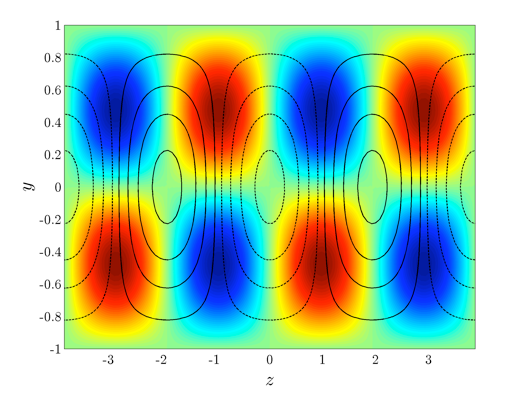 |
The most amplified sets of fluctuations are given by high (hot colors) and low (cold colors) streamwise velocities, with pairs of counter-rotating streamwise vortices in between them (contour lines). |