 nodes.
 % A 2D lattice example for the noise-corrupted leader-selection problem. % % form the incidence matrix and graph Laplacian matrix for 2D lattice % % number of nodes for the N x N 2D lattice n = 81; N = sqrt(n); % compute the number of edges ne = 0.5*( 2*4 + (N-2)*3*4 + (N-2)^2*4 ); % form the index set of edges idx = zeros(2,ne); % evaluate the indices for those edges on the rows of the grid for i = 1:N idx(1,(N-1)*(i-1)+1:(N-1)*i) = N*(i-1)+1:N*(i-1)+(N-1); idx(2,(N-1)*(i-1)+1:(N-1)*i) = N*(i-1)+2:N*(i-1)+N; end % evaluate the indices for those edges on the columns of the grid for i = 1:N idx(1,ne/2+ ((N-1)*(i-1)+1:(N-1)*i) ) = i:N:(i+(N-2)*N); idx(2,ne/2+ ((N-1)*(i-1)+1:(N-1)*i) ) = (i:N:(i+(N-2)*N))+N; end % form the incidence matrix Eg of the 2D lattice Eg = incmat(idx); % form the graph Laplacian L = Eg*Eg'; % kappa is taken as the diagonal of L kappa = diag(L); % Start solving the leader selection problem % % choose the number of leaders kval = 1:1:40; % pre-allocate memory for data collection Jlow = zeros(size(kval)); Jup = zeros(size(kval)); LSgreed = zeros(n,length(kval)); for i = 1:length(kval) Nl = kval(i); flag = 1; % for the noise-corrupted leader selection formulation [Jlow(i),Jup(i),LSgreed(:,i)] = leaders(L,Nl,kappa,flag); end
A 2D lattice
 |
We consider the noise-corrupted leader selection problem for a 2D regular lattice with |
Matlab code
Computational results
Download Matlab code lattice_example.m to reproduce these figures.
Performance bounds
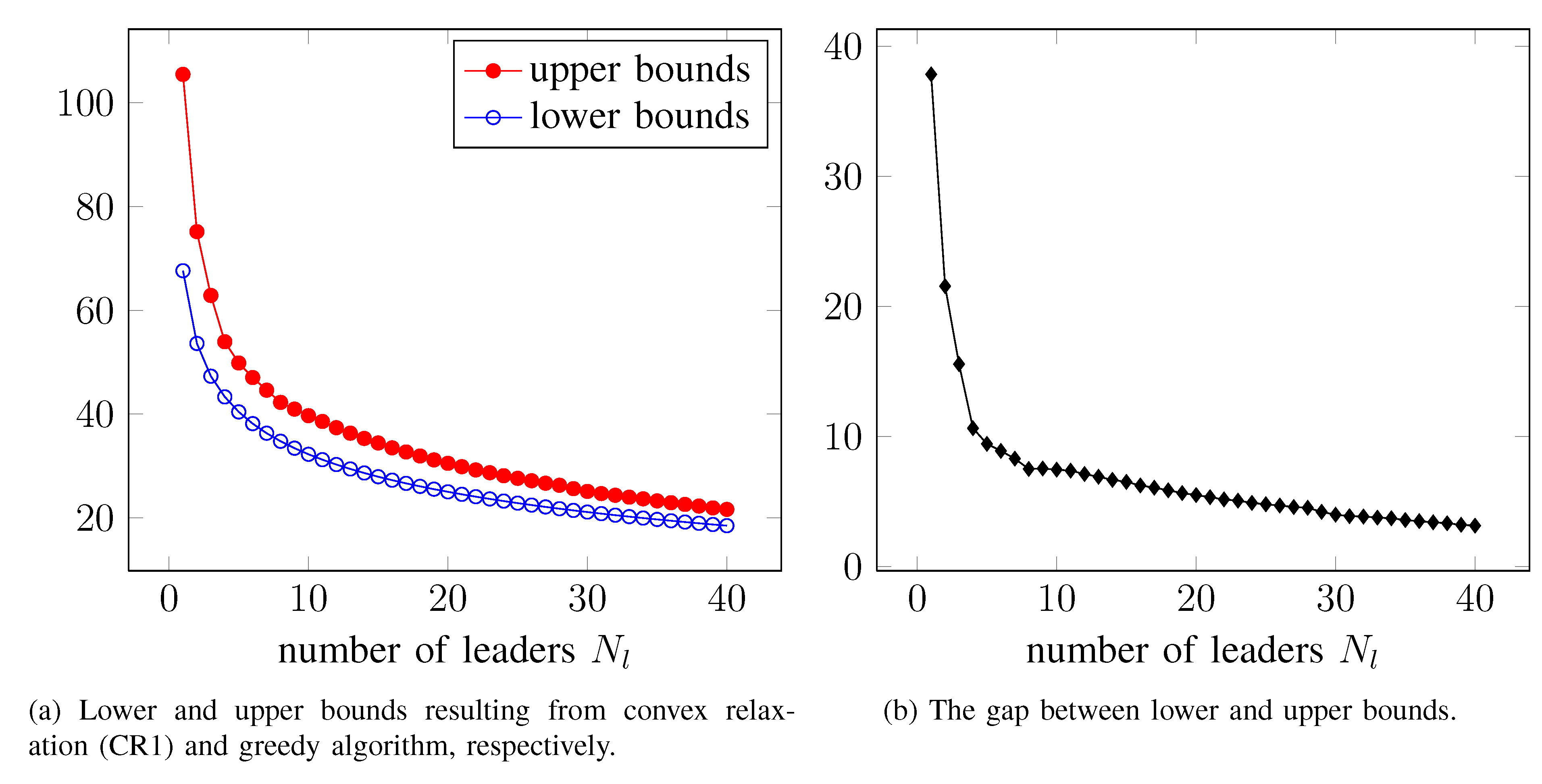 |
Bounds on the global optimal value of the noise-corrupted leader selection problem
 for the 2D lattice example.
Selection of leaders
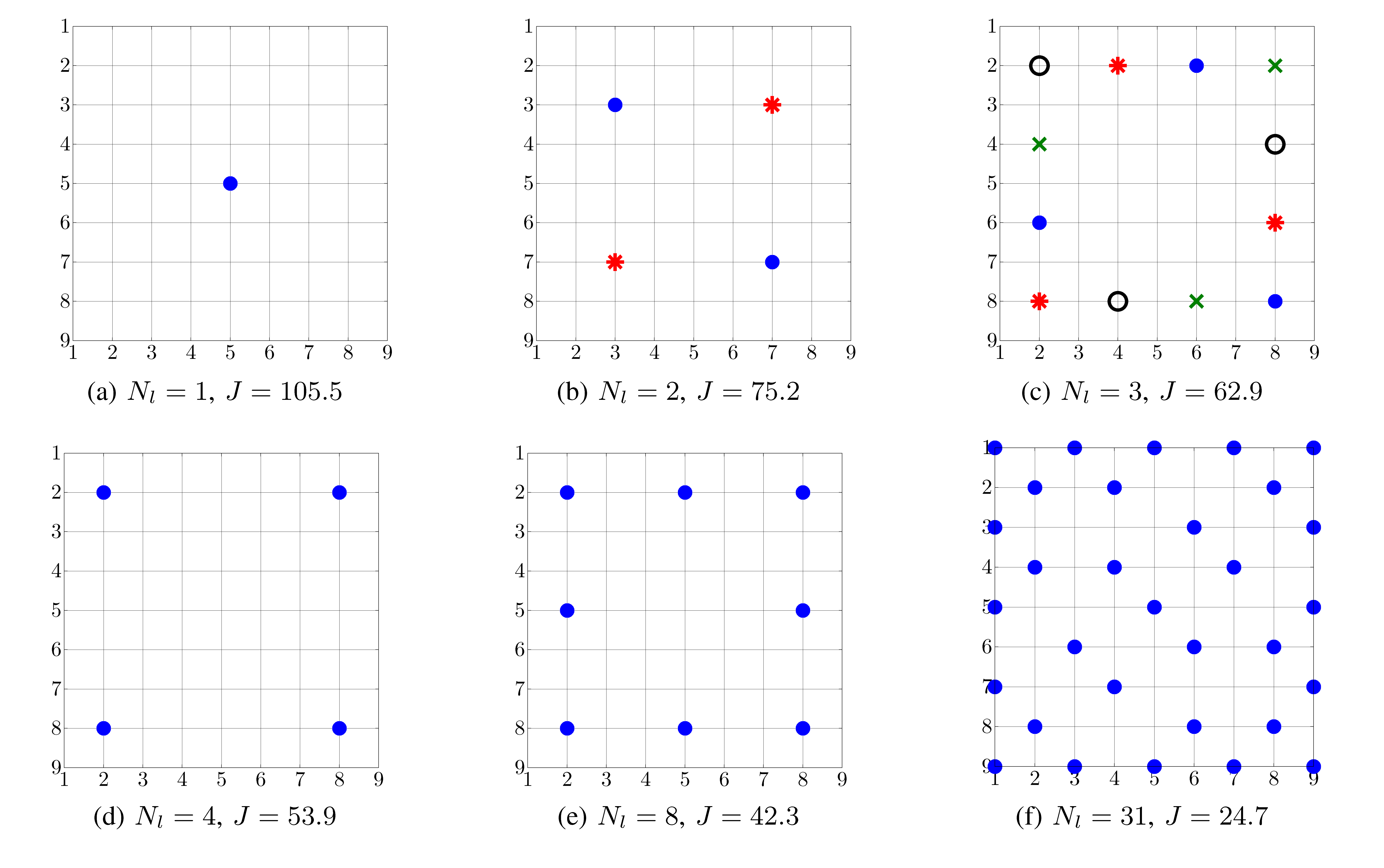 |
Selection of noise-corrupted leaders ( ) obtained using
greedy algorithm (i.e., one-leader-at-a-time algorithm followed by the swap procedure)
for the 2D lattice example.
) obtained using
greedy algorithm (i.e., one-leader-at-a-time algorithm followed by the swap procedure)
for the 2D lattice example.
For  , the center node
  provides the optimal
selection of a single leader. As
provides the optimal
selection of a single leader. As  increases, nodes away from the center
node are selected; for example, for
increases, nodes away from the center
node are selected; for example, for  , nodes
  ,
,  are
selected and for
are
selected and for  , nodes
  ,
,  ,
,  are selected.
Selection of nodes farther away from the center becomes more significant for
are selected.
Selection of nodes farther away from the center becomes more significant for
 and
and  .
.
The selection of leaders exhibits symmetry with respect to the center
of the lattice. For example, in Fig. (b), the leaders at  ,
,  denoted by
(
denoted by
( ) provide the same objective function
  as leaders denoted by (). Similarly,
in Fig. (c), the four selections of three leaders denoted by (), (),
(
as leaders denoted by (). Similarly,
in Fig. (c), the four selections of three leaders denoted by (), (),
( ), and (
 ) all provide the same performance .
Also note that when is large, almost uniform spacing between leaders is
observed; see Fig. (f). This is in contrast to the random network example where boundary nodes were selected when the number
of leaders is large.