Problem formulation
Noise-corrupted leader selection
We consider networks in which each node updates a scalar state  ,
,

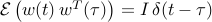
where  is the control input and
  is the white stochastic
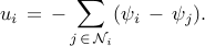
disturbance with zero-mean and unit-variance. A node is a follower if it
uses only relative information exchange with its neighbors to form its
control action,
is the white stochastic
disturbance with zero-mean and unit-variance. A node is a follower if it
uses only relative information exchange with its neighbors to form its
control action,
A node is a leader if, in addition to relative information exchange with
its neighbors, it also has access to its own state
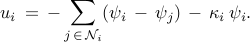
Here,  is a positive number and
  is the set of all
nodes that node
is the set of all
nodes that node  communicates with. A state-space representation of the
leader-follower consensus network is thus given by
communicates with. A state-space representation of the
leader-follower consensus network is thus given by

where  is a
Boolean-valued vector with its th entry
is a
Boolean-valued vector with its th entry  , indicating
that node is a leader if
, indicating
that node is a leader if  and that node is a follower if
 . The steady-state covariance matrix of
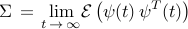
can be determined from the Lyapunov equation

where  is the expectation operator and
 .
The unique solution of the Lyapunov equation is given by
.
The unique solution of the Lyapunov equation is given by
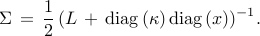
We use the total steady-state variance

to quantify deviation from consensus of stochastically forced networks.
Thus, the problem of identifying  leaders that are most effective in
reducing the mean-square deviation can be formulated as
leaders that are most effective in
reducing the mean-square deviation can be formulated as
![begin{array}{lrcl} {rm minimize} & J(x) & = & {rm trace} left( (L ,+, {rm diag} , (kappa) , {rm diag} , (x) )^{-1} right) [0.25cm] {rm subject~to} & x_i & in & {0,1}, ~~~~~ i ; = ; 1,ldots,n [0.15cm] & displaystyle{sum_{i , = , 1}^n} , x_i & = & N_l end{array} ~~~~~~~ ({rm LS1})](eqs/4333843790813906010-130.png)
where the graph Laplacian  and the vector
  with positive
elements are problem data, and the Boolean-valued vector with
cardinality
with positive
elements are problem data, and the Boolean-valued vector with
cardinality  is the optimization variable.
In sensor networks, it can be shown that  is equivalent to the
problem of choosing absolute position measurements among
is equivalent to the
problem of choosing absolute position measurements among  sensors in
order to minimize the variance of the estimation error; see
our paper for details.
sensors in
order to minimize the variance of the estimation error; see
our paper for details.
Noise-free leader selection
Since the leaders are subject to stochastic disturbances, we refer
to as the noise-corrupted leader selection problem. We
also consider the selection of noise-free leaders which follow their
desired trajectories at all times. Equivalently, in
coordinates that determine deviation from the desired trajectory, the state
of every leader is identically equal to zero, and the network dynamics are
thereby governed by the dynamics of the followers
Here,  is obtained from by eliminating all rows and columns
associated with the leaders.
is obtained from by eliminating all rows and columns
associated with the leaders.
Thus, the problem of selecting leaders that minimize the steady-state
variance of  amounts to
![begin{array}{lrcl} {rm minimize} & J_f(x) & = & {rm trace} , (L_f^{-1}) [0.25cm] {rm subject~to} & x_i & in & {0,1}, ~~~~~ i ; = ; 1,ldots,n [0.15cm] & displaystyle{sum_{i , = , 1}^n} , x_i & = & N_l end{array} ~~~~~~~ ({rm LS2})](eqs/6253127923021460596-130.png)
where the Boolean-valued vector with cardinality is the
optimization variable. The index set of nonzero elements of identifies
the rows and columns of the graph Laplacian that need to be deleted in
order to obtain . For example, for a path graph with three nodes,
assigning the center node as a noise-free leader implies that ![x ,=, [~0~1~0~]^T](eqs/6250791541045702417-130.png) . Thus,
deleting the
. Thus,
deleting the  nd row and column of the graph Laplacian
![L ;=; left[ begin{array}{rrr} 1 & -1 & 0 -1 & 2 & -1 0 & -1 & 1 end{array} right]](eqs/7496899904124718758-130.png)
yields the corresponding principal submatrix
![L_f ;=; left[ begin{array}{rr} 1 & 0 0 & 1 end{array} right].](eqs/5889618049295484763-130.png)
Since the objective function  in
in  is not expressed
explicitly in terms of the optimization variable , it is difficult to
examine its basic properties including convexity. In
our paper, we show that
is not expressed
explicitly in terms of the optimization variable , it is difficult to
examine its basic properties including convexity. In
our paper, we show that  can be
equivalently written as
can be
equivalently written as

where  is the elementwise multiplication of two matrices and
  is the vector of all ones.
Finally, in sensor networks, it can be shown that amounts
to choosing sensors with a priori known positions such that the
variance of the estimation error is minimized; see
our paper for details.