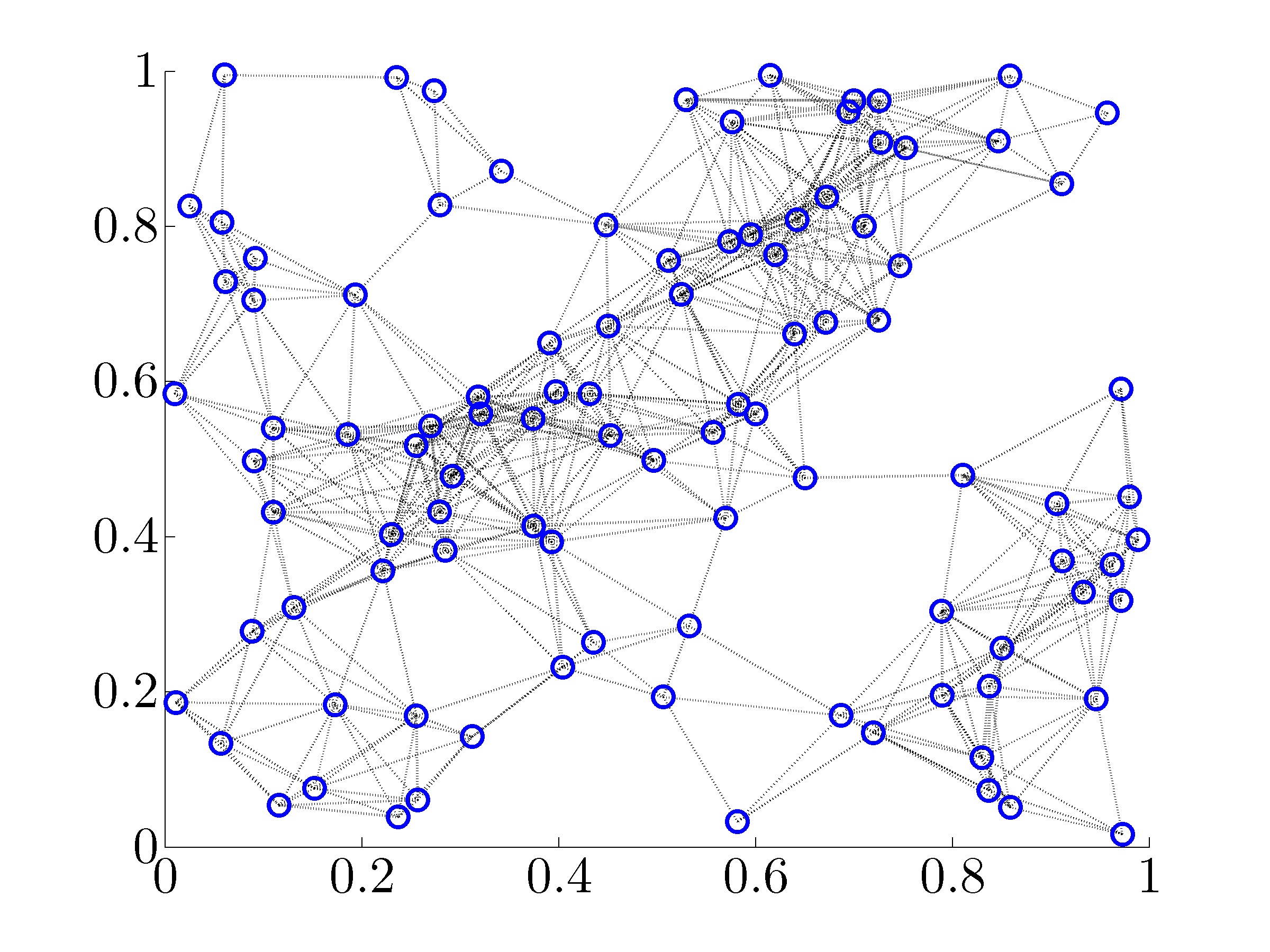
 randomly distributed nodes in a unit square. A pair of nodes communicate
with each other if their distance is not greater than
randomly distributed nodes in a unit square. A pair of nodes communicate
with each other if their distance is not greater than  units. This
scenario may arise in sensor networks with prescribed omnidirectional (i.e.,
disk shape) sensing range.
units. This
scenario may arise in sensor networks with prescribed omnidirectional (i.e.,
disk shape) sensing range. % Generate 100 nodes randomly distributed in a square of Length x Length units n = 100; % load the position data load position.mat Length = 1; % Or generate a new set of position data % position = Length*rand(n,2); % radius that determines the neighbors of nodes r = Length/5; % draw neighbors and compute the incidence matrix of neighboring nodes [Eg,idx] = neighbors(n,position,r); % form the graph Laplacian L = Eg*Eg'; % kappa is taken as the diagonal of L kappa = diag(L); % Start solving the leader selection problem kval = 1:1:40; % pre-allocate memory for data collection Jlow = zeros(size(kval)); Jup = zeros(size(kval)); LSgreed = zeros(n,length(kval)); for i = 1:length(kval) Nl = kval(i); flag = 1; % for noise-corrupted leader selection formulation [Jlow(i),Jup(i),LSgreed(:,i)] = leaders(L,Nl,kappa,flag); end
A random network
 |
We consider the selection of noise-corrupted leaders in a network with
|
Matlab code
Computational results
Download Matlab code random_network_example.m to reproduce these figures.
Performance bounds
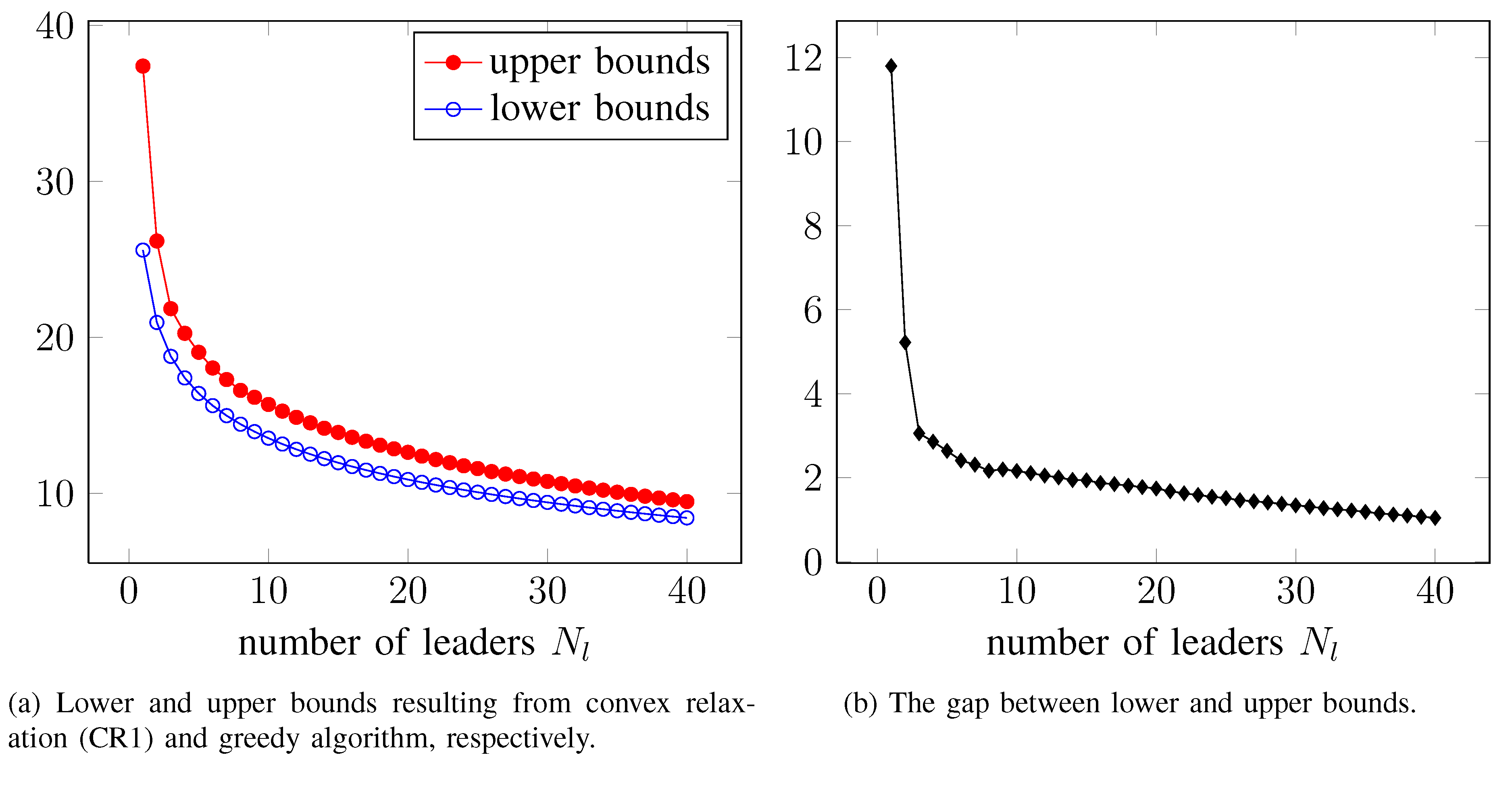 |
Bounds on the global optimal value of the noise-corrupted
leader selection problem ( ) for the random network example.
Greedy algorithm vs. degree heuristics
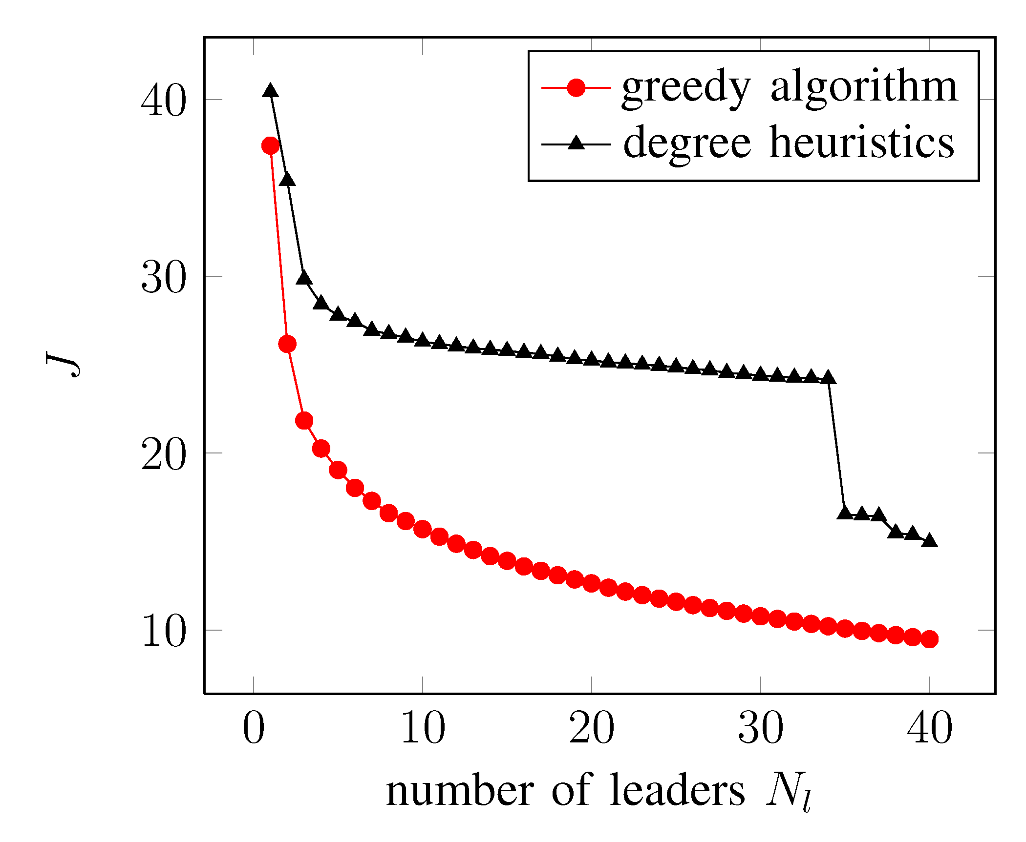 |
Greedy algorithm (i.e., one-leader-at-a-time algorithm followed by the swap procedure) significantly outperforms degree heuristics (that selects leaders with the largest number of neighbors) for the random network example. To gain some insight into the selection of leaders, we compare results obtained using the greedy algorithm with degree heuristics. |
 |
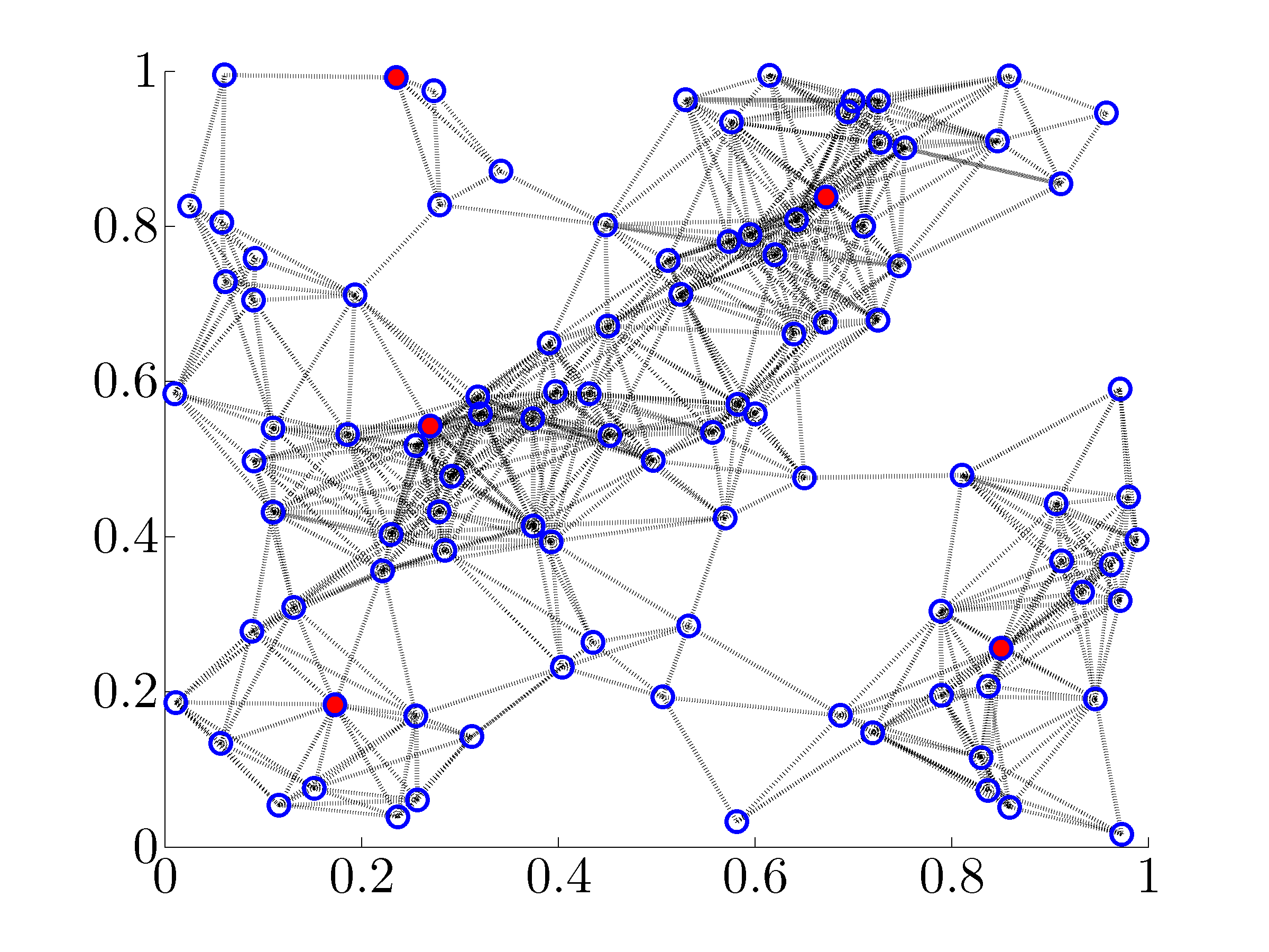
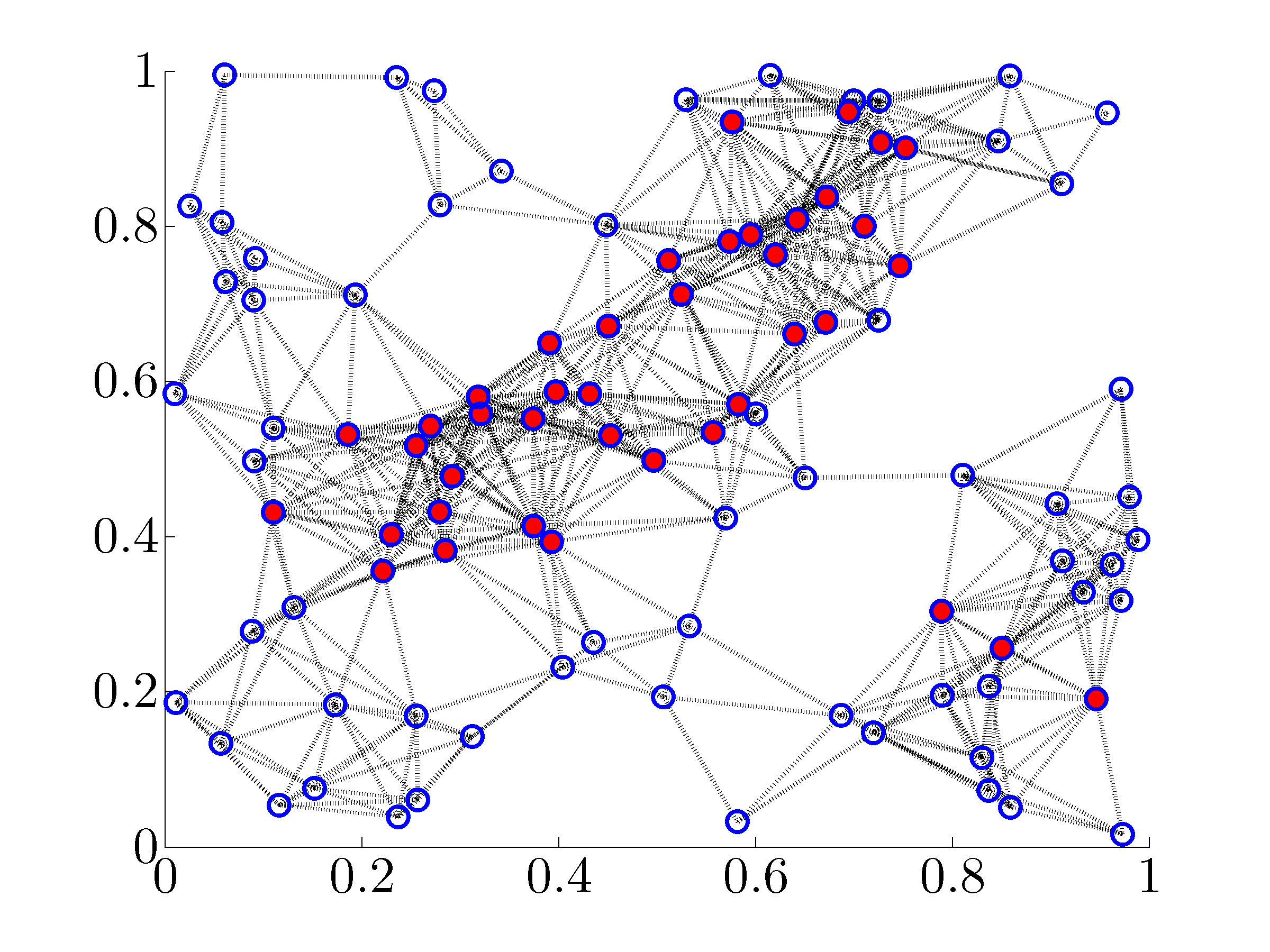
Selection of |
 noise-corrupted leaders using degree heuristics.
 .
.
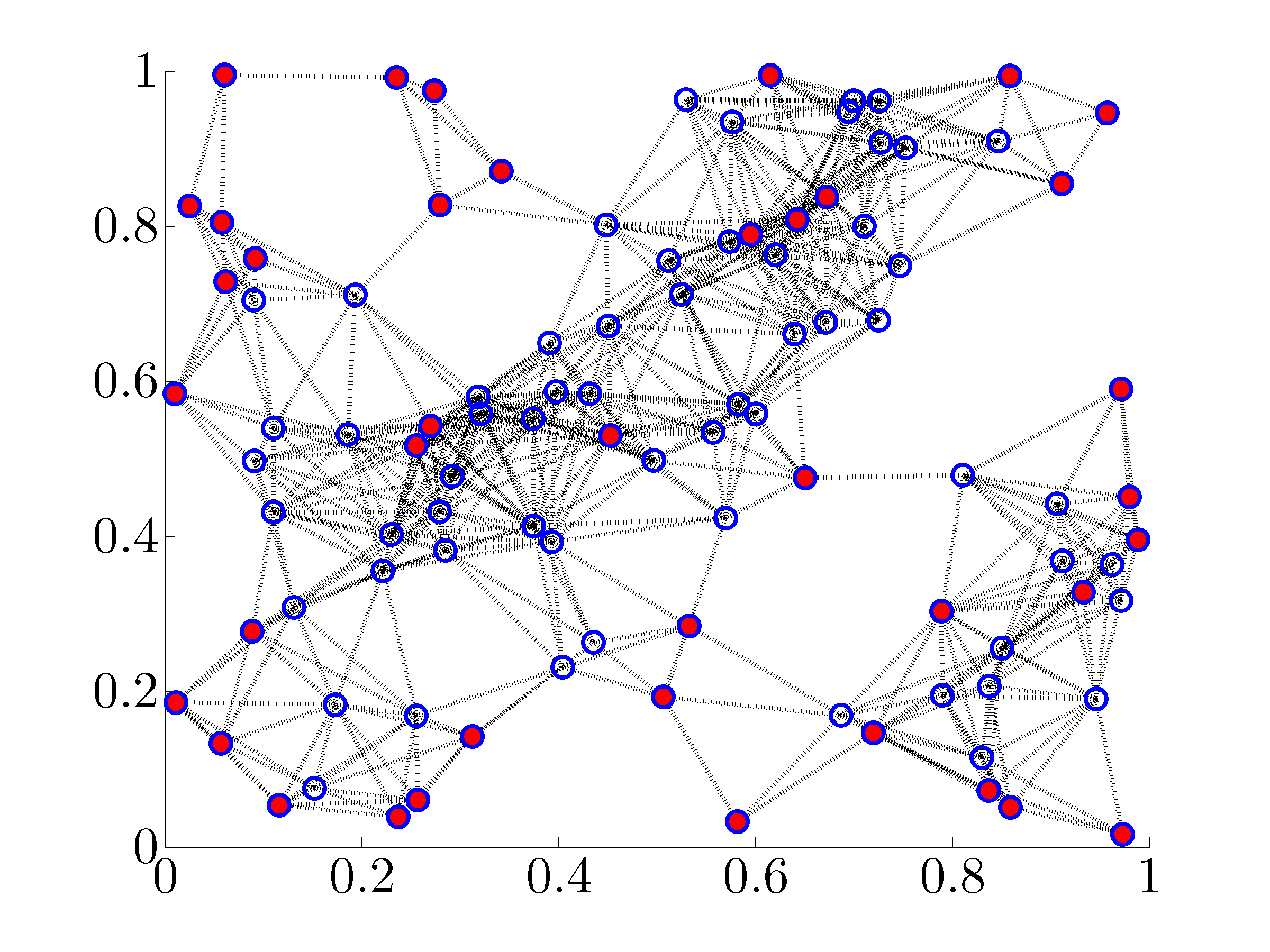
 |
Selection of |
 .
.
 |
Selection of |
 noise-corrupted leaders using degree heuristics.
 .
.
 |
Selection of |
 .
.