 nodes are randomly and uniformly distributed in a square region of
  units.
Each node is an unstable second order linear system coupled with other nodes through the following dynamics
units.
Each node is an unstable second order linear system coupled with other nodes through the following dynamics
 and
and  is determined by
the Euclidean distance
is determined by
the Euclidean distance  between them. The performance weights
 and
and  are set to identity matrices.
% An example from Motee and Jadbabaie,
% "Optimal control of spatially distributed systems",
% IEEE Trans. Automat. Control,
% vol. 53, no. 7, pp. 1616–1629, 2008.

% N nodes randomly distributed in a box [0 L] x [0 L]
N = 100;
L = 10;

load data/positions
% or generate the random distribution of the nodes
% pos = L*rand(N,2);

% the state-space representation of subsystem i
Aii = [1 1; 1 2];
Bii = [0; 1];
n   = size(Bii,1);
Aij = eye(n);

B1  = kron(eye(N), Bii);
B2  = B1;

% construct
% (a) the Euclidean distance matrix that describes the distance
% between two systems i and j
% (b) the A-matrix of the distributed system

A = zeros(2*N,2*N);
dismat = zeros(N,N);
for i = 1:N
    for j = i:N
        if i == j
            A( (i-1)*n + 1 : i*n, (j-1)*n + 1 : j*n ) = Aii;
        else
            dismat(i,j) = sqrt( norm( pos(i,:) - pos(j,:) )^2 );
            dismat(j,i) = dismat(i,j);
            A( (i-1)*n + 1 : i*n, (j-1)*n + 1 : j*n ) = Aij / exp( dismat(i,j) );
            A( (j-1)*n + 1 : j*n, (i-1)*n + 1 : i*n ) = Aij / exp( dismat(j,i) );
        end
    end
end

% state and control penalty weights
Q = eye(2*N);
R = eye(N);

% compute sparse feedback gains
options = struct('method','wl1','gamval',logspace(-2,log10(68.6649),48), ...
        'rho',100,'maxiter',10,'blksize',[1 1],'reweightedIter',1);

tic
solpath = lqrsp(A,B1,B2,Q,R,options);
toc
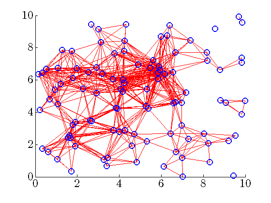
Network with 100 unstable nodes
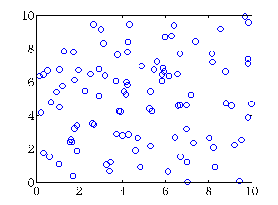 |
![begin{array}{rcccccc} left[ begin{array}{c} dot{p}_i dot{v}_i end{array} right] & ! = ! & underbrace{left[ begin{array}{cc} {1} & {1} {1} & {2} end{array} right] left[ begin{array}{c} {p_i} {v_i} end{array} right]}_{ begin{array}{c} mbox{bf unstable} [0.1cm] mbox{bf dynamics} end{array} } & ! + ! & underbrace{sum_{j , neq , i} ; mathrm{e}^{-{alpha (i,j)}} left[ begin{array}{c} {p_j} {v_j} end{array} right]}_{mbox{bf coupling}} & ! + ! & left[ begin{array}{c} {0} {1} end{array} right] left( d_i ; + ; u_i right). end{array}](eqs/2090195765460056142-130.png)
The coupling between two nodes |
We next present the Matlab code and the computational results obtained
using lqrsp.m. In this example, we use the weighted  norm to promote
sparsity. We set
norm to promote
sparsity. We set  ,
,  and select
  logarithmically-spaced
points for
logarithmically-spaced
points for ![gamma in [0.01, , 68.66]](eqs/5299860170265800376-130.png) .
.
Matlab code
Computational results
Download Matlab code spatially_dist.m to reproduce these figures.
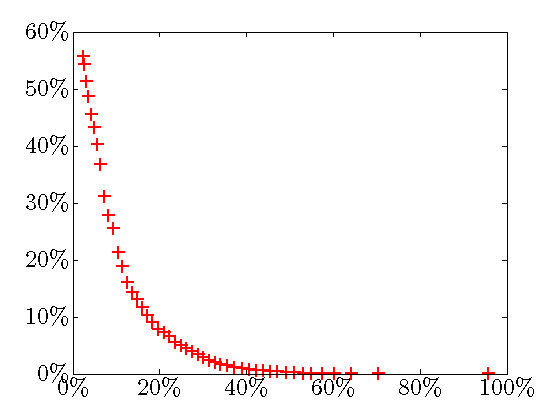
Sparsity vs. performance
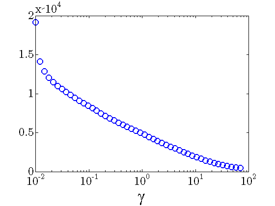 |
Number of nonzero elements in the feedback gain decreases with |
In the absence of sparsity constraints, i.e., at  , the optimal
  controller
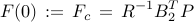
is obtained from the positive definite solution of the algebraic Riccati equation

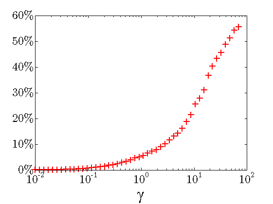 |
Performance loss:
|
 |
Sparsity level:
|
 -axis) vs. Sparsity level (
 -axis);
Sparsity vs. performance
![begin{array}{cccc} gamma & 12.6 & 26.8 & 68.7 [0.35cm] displaystyle{frac{ {rm bf{card}} , (F) }{ {rm bf{card}} , (F_{c}) }} & {bf 8.3} % & 4.9 % & 2.4 % [0.5cm] displaystyle{ frac{J(F) ,-, J(F_c)}{J(F_c)} } & {bf 27.8} % & 43.3 % & 55.6 % end{array}](eqs/3350296090378245433-130.png)
The above results demonstrate that the optimal sparse feedback gain,
with  of non-zero elements relative to the centralized feedback gain
  ,
introduces performance loss of
,
introduces performance loss of  compared to .
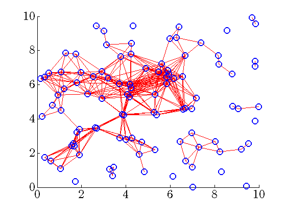
Communication graphs of distributed controllers
As  increases, the communication architecture of distributed controllers becomes sparser.
Note that the communication graph does not have to be connected since the subsystems are
increases, the communication architecture of distributed controllers becomes sparser.
Note that the communication graph does not have to be connected since the subsystems are
dynamically coupled to each other;
allowed to measure their own states.
 |
Communication graph of the distributed controller for
![begin{array}{rcl} gamma & = & 12.6486 [0.25cm] displaystyle{frac{ {rm bf{card}} , (F) }{ {rm bf{card}} , (F_{c}) }} times 100 % & = & 8.3% [0.5cm] displaystyle{frac{J(F) ,-, J(F_c)}{J(F_c)}} times 100 % & = & 27.8%. end{array}](eqs/8219290527741224301-130.png)
|
 |
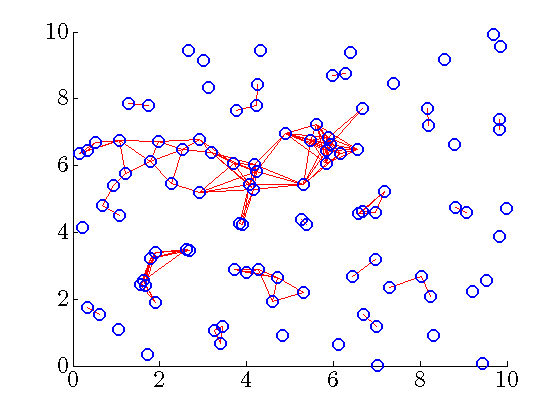
Communication graph of the distributed controller for ![begin{array}{rcl} gamma & = & 26.8270 [0.25cm] displaystyle{frac{ {rm bf{card}} , (F) }{ {rm bf{card}} , (F_{c}) }} times 100 % & = & 4.9% [0.5cm] displaystyle{frac{J(F) ,-, J(F_c)}{J(F_c)}} times 100 % & = & 43.3%. end{array}](eqs/241735647017072518-130.png)
|
 |
Communication graph of the distributed controller for ![begin{array}{rcl} gamma & = & 68.6649 [0.25cm] displaystyle{frac{ {rm bf{card}} , (F) }{ {rm bf{card}} , (F_{c}) }} times 100 % & = & 2.4% [0.5cm] displaystyle{frac{J(F) ,-, J(F_c)}{J(F_c)}} times 100 % & = & 55.6%. end{array}](eqs/3240235551264210185-130.png)
|
Danger of truncation
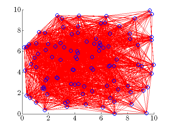 |
Our sparsity-promoting algorithm identifies communication architectures that are difficult to
guess a priori. To highlight this point, and to illustrate danger of truncation, let us consider
the truncated centralized gain ![(F_t)_{ij} , := , left{ begin{array}{ll} 0 & {rm if}~ |(F_c)_{ij}| , < , a [0.2cm] (F_c)_{ij} & {rm if}~ |(F_c)_{ij}| , geq , a. end{array} right.](eqs/8907536851530871033-130.png)
The figure shows the communication graph of the truncated controller obtained by setting |
 ,
,  .
Even though the communication graph appears to be very dense (
.
Even though the communication graph appears to be very dense ( nonzero elements —
  relative to
  ), the truncated gain does not even provide the closed-loop stability.