Wide Area Control of IEEE 39 New England Power Grid Model
 |
Contributed by Florian Dorfler and Mihailo R. Jovanovic Matlab Files
Presentations
Papers
|
Problem description
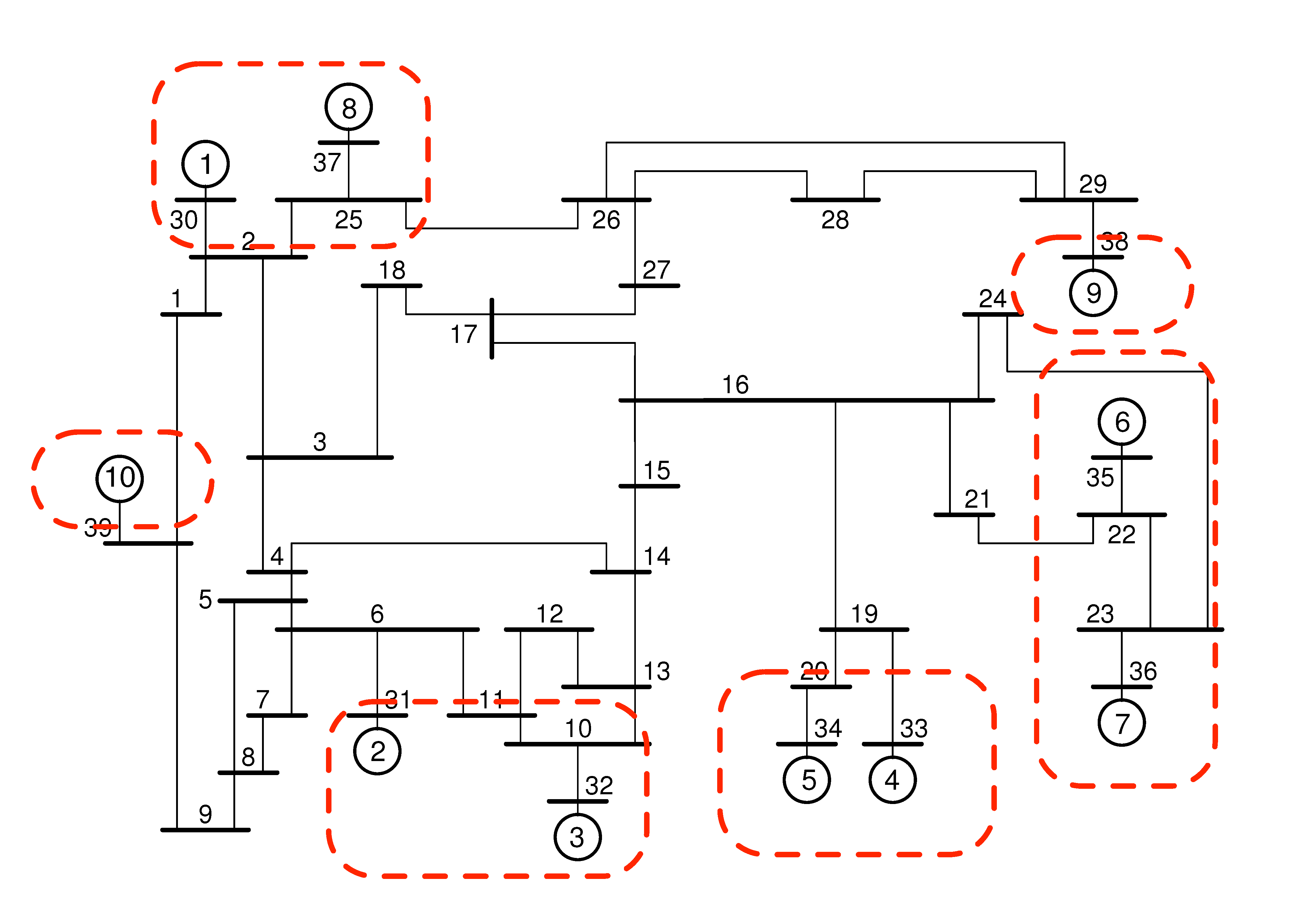
The IEEE  New England Power Grid Model consists of buses and
 generators. Generator is an equivalent aggregated model for
the part of the network that we do not have control over; generators
generators. Generator is an equivalent aggregated model for
the part of the network that we do not have control over; generators  to
to  are equipped with Power System Stabilizers (PSSs), which provide
good damping of local modes and stabilize otherwise unstable open-loop
system. We use a sparsity-promoting optimal control strategy to design a
supplementary wide area control signal aimed at achieving a desirable
trade-off between damping of the inter-area oscillations and
communication requirements in the distributed controller. Inter-area
oscillations are associated with the dynamics of power transfers and
they are characterized by groups of coherent machines that swing
relative to each other. These oscillations are caused by weakly damped
modes of the linearized swing equations and they physically correspond
to active power transfer between different generator groups.
are equipped with Power System Stabilizers (PSSs), which provide
good damping of local modes and stabilize otherwise unstable open-loop
system. We use a sparsity-promoting optimal control strategy to design a
supplementary wide area control signal aimed at achieving a desirable
trade-off between damping of the inter-area oscillations and
communication requirements in the distributed controller. Inter-area
oscillations are associated with the dynamics of power transfers and
they are characterized by groups of coherent machines that swing
relative to each other. These oscillations are caused by weakly damped
modes of the linearized swing equations and they physically correspond
to active power transfer between different generator groups.
In the absence of higher-order generator dynamics, for purely inductive lines and constant-current loads, the dynamics of each generator can be represented by the electromechanical swing equations
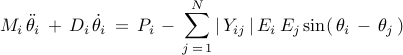
where  denotes the number of generators,
  is the generator power
injection in the network-reduced model, and
is the generator power
injection in the network-reduced model, and  is the Kron-reduced
admittance matrix describing the interactions among generators. After
linearization at an operating point the swing equations reduce to
is the Kron-reduced
admittance matrix describing the interactions among generators. After
linearization at an operating point the swing equations reduce to
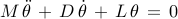
where  and
and  are diagonal matrices of inertia and damping
coefficients, and the coupling among generators is entirely described
by the weighted graph induced by the Laplacian matrix
are diagonal matrices of inertia and damping
coefficients, and the coupling among generators is entirely described
by the weighted graph induced by the Laplacian matrix  .
.
Let the state of the power network be partitioned as ![x , = , [ ~~ theta^T quad dot{theta}^T quad x_{rm rem}^T ~~ ]^T](eqs/8949456625638288486-130.png) where
where  and
and  are the rotor angles and frequencies of
synchronous generators and
are the rotor angles and frequencies of
synchronous generators and  are the state variables which
correspond to fast electrical dynamics.
are the state variables which
correspond to fast electrical dynamics.
The sparsity-promoting minimum-variance optimal control problem can then be formulated as:
![begin{array}{rrcl} mbox{bf linearized dynamics:} & dot{x}(t) & = & A , x(t) ,+, B_1 , d(t) ,+, B_2 , u(t) [0.35cm] mbox{bf objective function:} & J & = & displaystyle{lim_{t ; to ; infty}} {cal E} left( theta^{T} (t) , Q_{theta} , theta(t) ,+, dot{theta}^{T} (t) , Q_{dot{theta}} , dot{theta} (t) ,+, u^{T} (t) , R , u(t) ,+, gamma , displaystyle{sum_{i, , j}} , w_{ij} , |F_{ij}| right) [0.6cm] mbox{bf memoryless controller:} & u & = & -F , x(t) end{array}](eqs/3340379952653995854-130.png)
where we use the weighted  norm to induce sparsity in the state
feedback gain matrix
norm to induce sparsity in the state
feedback gain matrix  .
.
Computational results
We next present computations resulting from the use of the
sparsity-promoting framework with  logarithmically-spaced points for
![gamma in [ , 10^{-4},, 1 , ]](eqs/6989932445942136790-130.png) . In the objective function we
choose
. In the objective function we
choose  ,
,  , and set
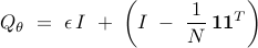
in order to penalize deviation from synchrony. This choice of
 is inspired by slow coherency theory with
  denoting a small regularization parameter and
  denoting the
vector of all ones.
denoting the
vector of all ones.
Download Matlab code neWAC.m and data file neData.mat to reproduce these figures.
Performance vs Sparsity
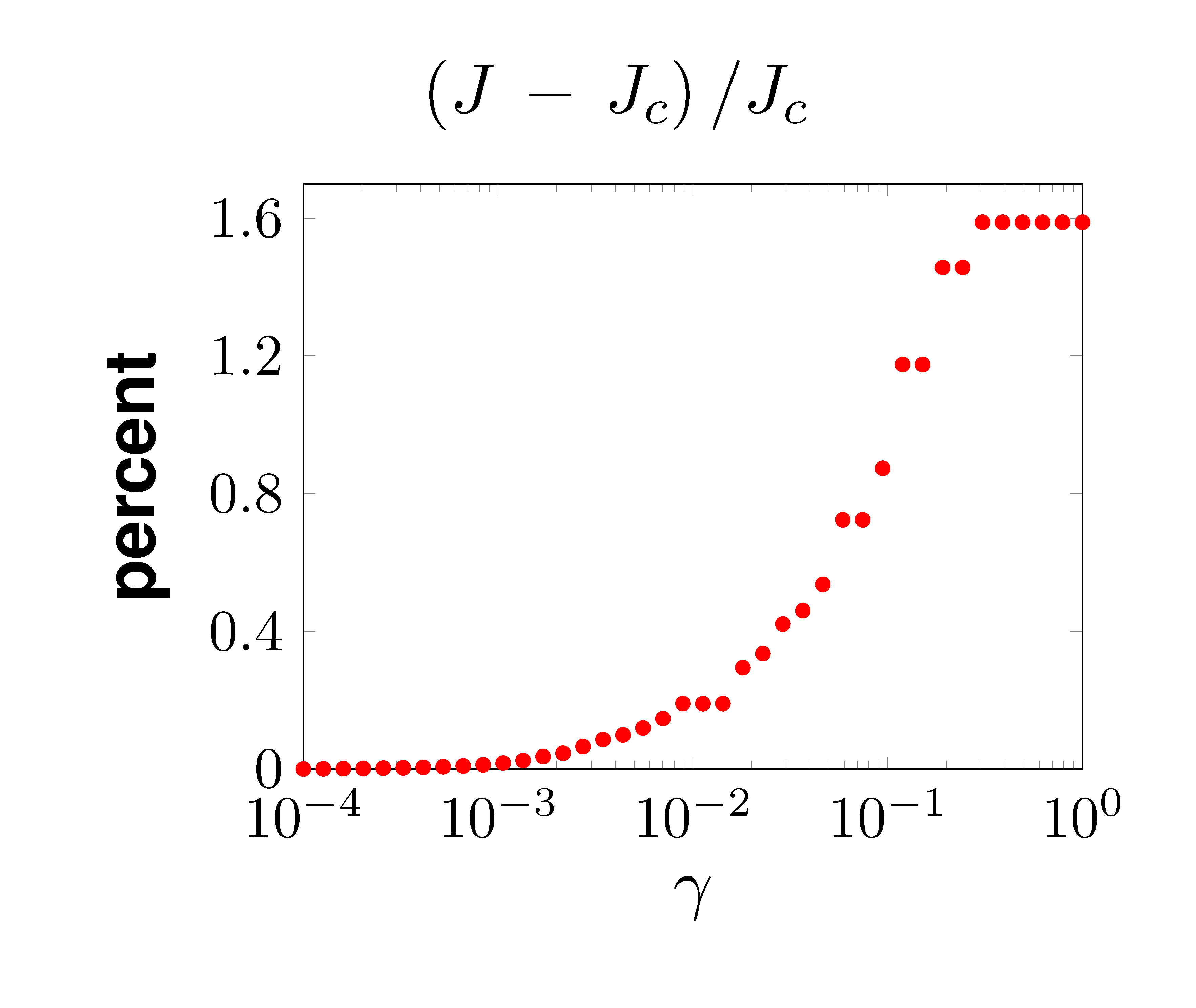 |
Relative to the optimal centralized controller, performance of the optimal sparse controller deteriorates gracefully with increased emphasis on sparsity. |
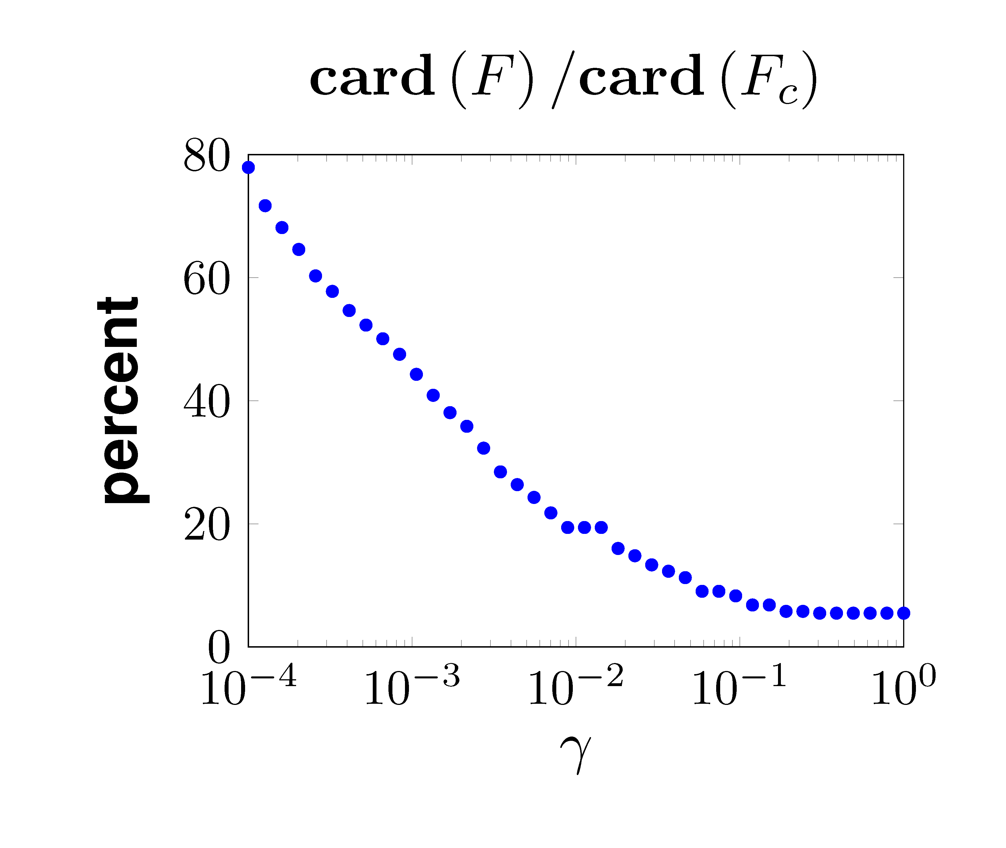 |
For Increased emphasis on sparsity induces feedback gains with smaller number of nonzero elements. |
 , the optimal centralized feedback gain
  is
a dense matrix populated with nonzero elements.
is
a dense matrix populated with nonzero elements.Signal exchange network
The sparsity pattern of the optimal feedback gain illustrates interactions between different generators. In the figures below, nine rows correspond to nine control inputs to controlled generators; the columns correspond to different states variables. Blue dots in each block represent local interactions within each generator, and red dots represent interactions between different generators.
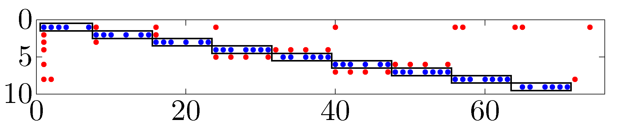 |
Identified long range interactions are represented by red dots. The optimal sparse controller promotes the use of angles and frequencies (i.e., the first and second states of each subsystem) as signals to be communicated. |
 ,
, 
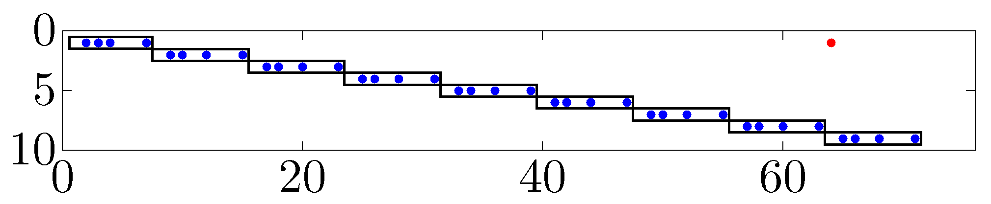 |
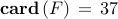
Only a single long range interaction is identified:
the controller at generator Relative to the optimal centralized feedback gain, the resulting
sparse controller degrades performance by only |
 ,
, 
 .
. .
.
 |
As our emphasis on sparsity increases, most of the control burden is on
generator |
 , only the angle of loosely connected
generator
, only the angle of loosely connected
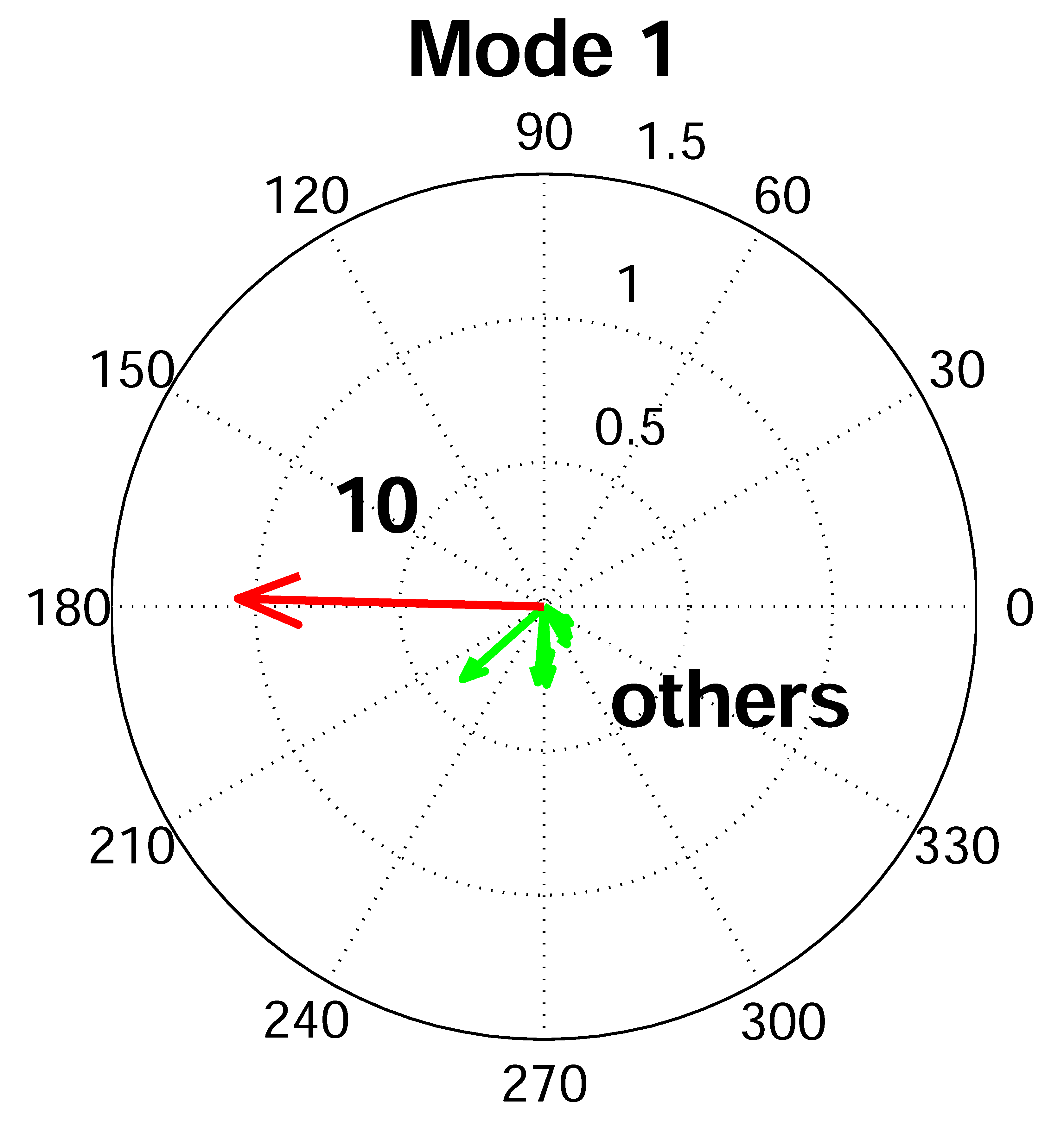
generator Dominant inter-area modes
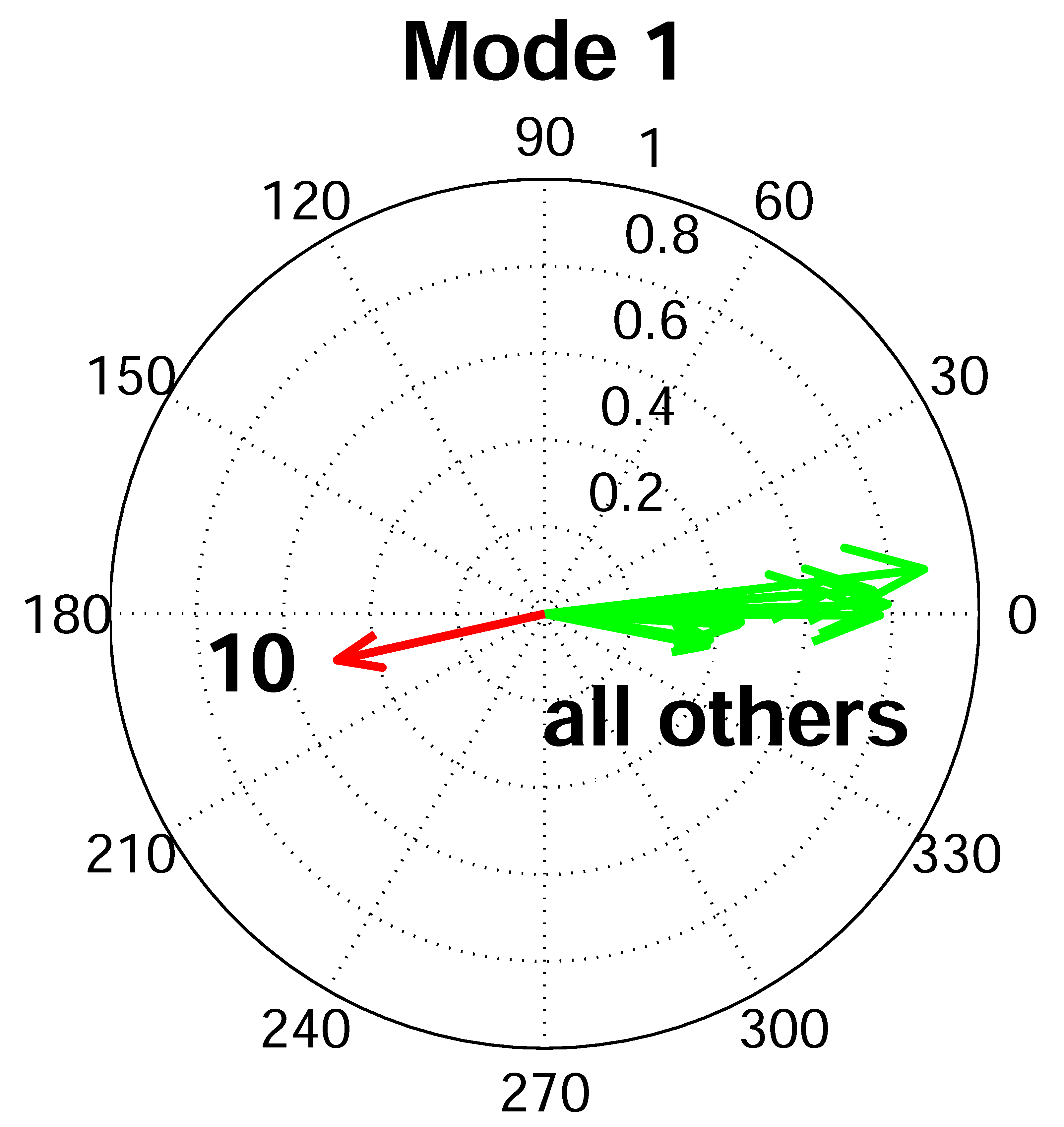 |
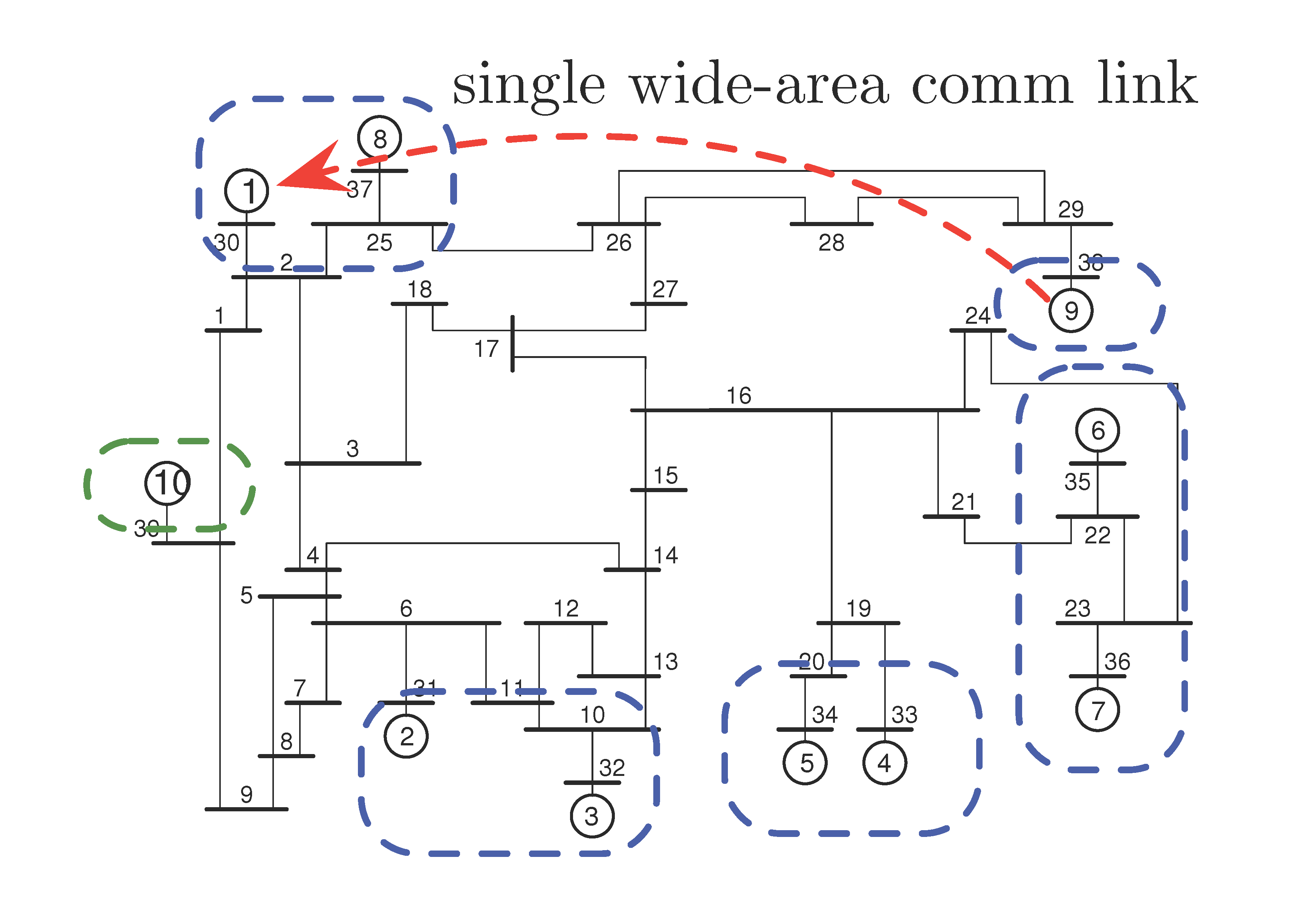
The polar plots show the generator frequency components of one of the poorly damped inter-area modes in the open-loop system (i.e., the system controlled with only local PSSs). This inter-area mode is characterized by active power transfer between
generator |
 |
The least damped inter-area mode of the closed-loop system (i.e., the
system controlled with both local PSSs and the optimal sparse wide-area
controller obtained for Relative to the open-loop system, the closed-loop system is
characterized by much smaller active power transfer between generator
|
 ).
). Presentations
Slow coherency and sparsity-promoting optimal wide-area control
Los Alamos National Lab
Los Alamos, NM; July 2013Sparsity-promoting wide-area control of power systems
2013 American Control Conference
Washington, DC; June 2013
Publications
Sparsity-promoting optimal wide-area control of power networks
F. Dorfler, M. R. Jovanovic, M. Chertkov, and F. Bullo
IEEE Trans. Power Syst., vol. 29, no. 5, pp. 2281-2291, 2014.Sparse and optimal wide-area damping control in power networks
F. Dorfler, M. R. Jovanovic, M. Chertkov, and F. Bullo
2013 American Control Conference, pp. 4295-4300, Washington DC, June 2013.
Citation
If you are using information provided here in your research or teaching,
please include explicit mention of this website
www.umn.edu/~mihailo/software/lqrsp/
and of our papers.
@article{dorjovchebulTPS14,
   author  = {F. D\"orfler and M. R. Jovanovi\'c and M. Chertkov and F. Bullo},
   title   = {Sparsity-promoting optimal wide-area control of power networks},
   journal = {IEEE Trans. Power Syst.},
   volume  = {29},
   number  = {5},
   pages   = {2281-2291},
   year    = {2014}
}

@inproceedings{dorjovchebulACC13,
   author       = {F. D\"orfler and M. R. Jovanovi\'c and M. Chertkov and F. Bullo},
   booktitle    = {Proceedings of the 2013 American Control Conference},
   title        = {Sparse and optimal wide-area damping control in power networks},
   year         = {2013},
   address      = {Washington, DC},
   pages        = {4295-4300}
}

@article{linfarjovADMM13,
   author  = {F. Lin and M. Fardad and M. R. Jovanovi\'c},
   title   = {Design of optimal sparse feedback gains via the alternating direction method of multipliers},
   journal = {IEEE Trans. Automat. Control},
   volume  = {58},
   number  = {9},
   pages   = {2426-2431},
   year    = {2013}
}