 masses on a line.
% Mass-spring system

% State-space representation of the mass-spring system with N = 50 masses
N = 50;
I = eye(N,N);
Z = zeros(N,N);
T = toeplitz([2 -1 zeros(1,N-2)]);
A = [Z I; -T Z];
B1 = [Z; I];
B2 = [Z; I];
Q = eye(2*N);
R = 10*I;

% Compute the optimal sparse feedback gains
options = struct('method','wl1','gamval',logspace(-4,-1,50),...
        'rho',100,'maxiter',100,'blksize',[1 1],'reweightedIter',5);
tic
solpath = lqrsp(A,B1,B2,Q,R,options);
toc
Mass-spring system: weighted  norm
norm
 |
Mass-spring system with |
The weighted  norm is given by
Since

we use the re-weighted scheme of Candes et al. ’08
where  is the optimal sparse feedback gain from the previous re-weighted
iteration.
is the optimal sparse feedback gain from the previous re-weighted
iteration.
At  , the solution of the optimal control problem is computed from
the positive definite solution of the algebraic Riccati equation. For a fixed
value of
, the solution of the optimal control problem is computed from
the positive definite solution of the algebraic Riccati equation. For a fixed
value of  , we initialize the re-weighted scheme using the
solution from the previous value of
, we initialize the re-weighted scheme using the
solution from the previous value of  . We update the weights until
convergence or a maximum number of iterations is reached.
. We update the weights until
convergence or a maximum number of iterations is reached.
We next show the Matlab code and the computational results obtained
using lqrsp.m. We set  and select
  logarithmically-spaced
points for
logarithmically-spaced
points for ![gamma in [10^{-4}, , 10^{-1}]](eqs/6525947523514546497-130.png) .
.
Matlab code
Computational results
Download Matlab code mass_spring_wl1.m to reproduce these figures.
Sparsity patterns
The number of nonzero elements in decreases with .
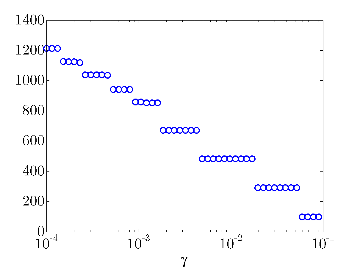 |
The number of nonzero elements in the feedback gain |
 masses, there are total of
  elements in
 The number of nonzero sub-diagonals in both position and velocity feedback gains
![F = [F_p ; ; F_v]](eqs/3382737894141789894-130.png) decreases with
decreases with  For large values of both
  and
and  become
diagonal matrices.
become
diagonal matrices.
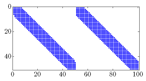 |
Sparsity pattern of the feedback gain matrix |
 .
.
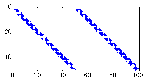 |
Sparsity pattern of the feedback gain matrix |
 .
.
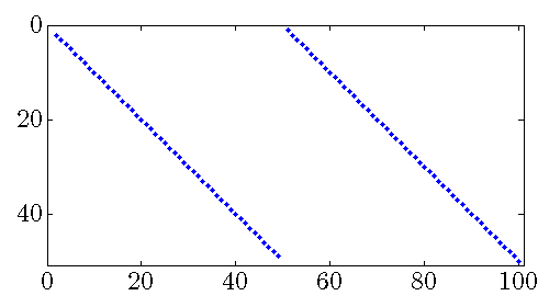 |
Sparsity pattern of the feedback gain matrix |
 .
.Performance of sparse feedback gains
In the absence of sparsity constraints, i.e., at , the optimal  controller
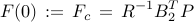
is obtained from the positive definite solution of the algebraic Riccati equation

As increases, the feedback gain becomes sparser and the quadratic
performance deteriorates.
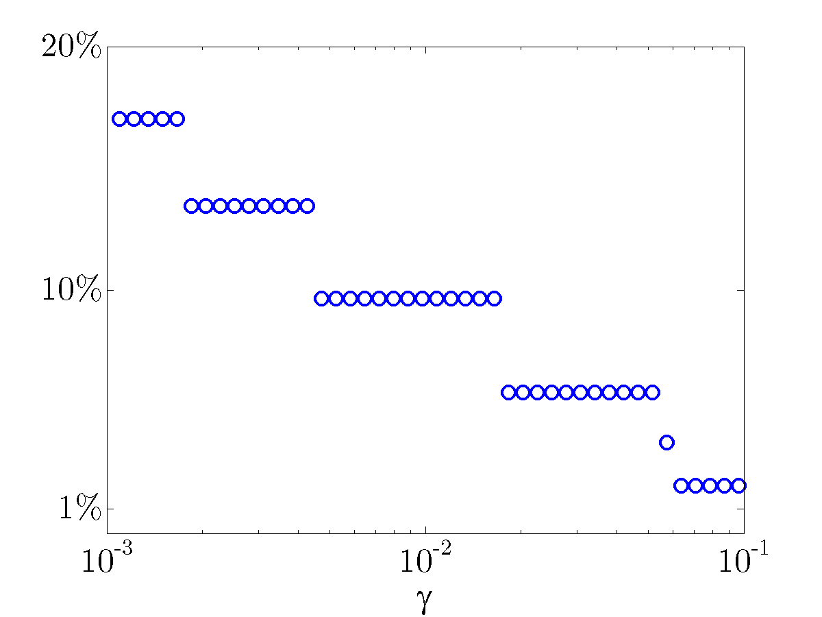 |
Sparsity level:
|
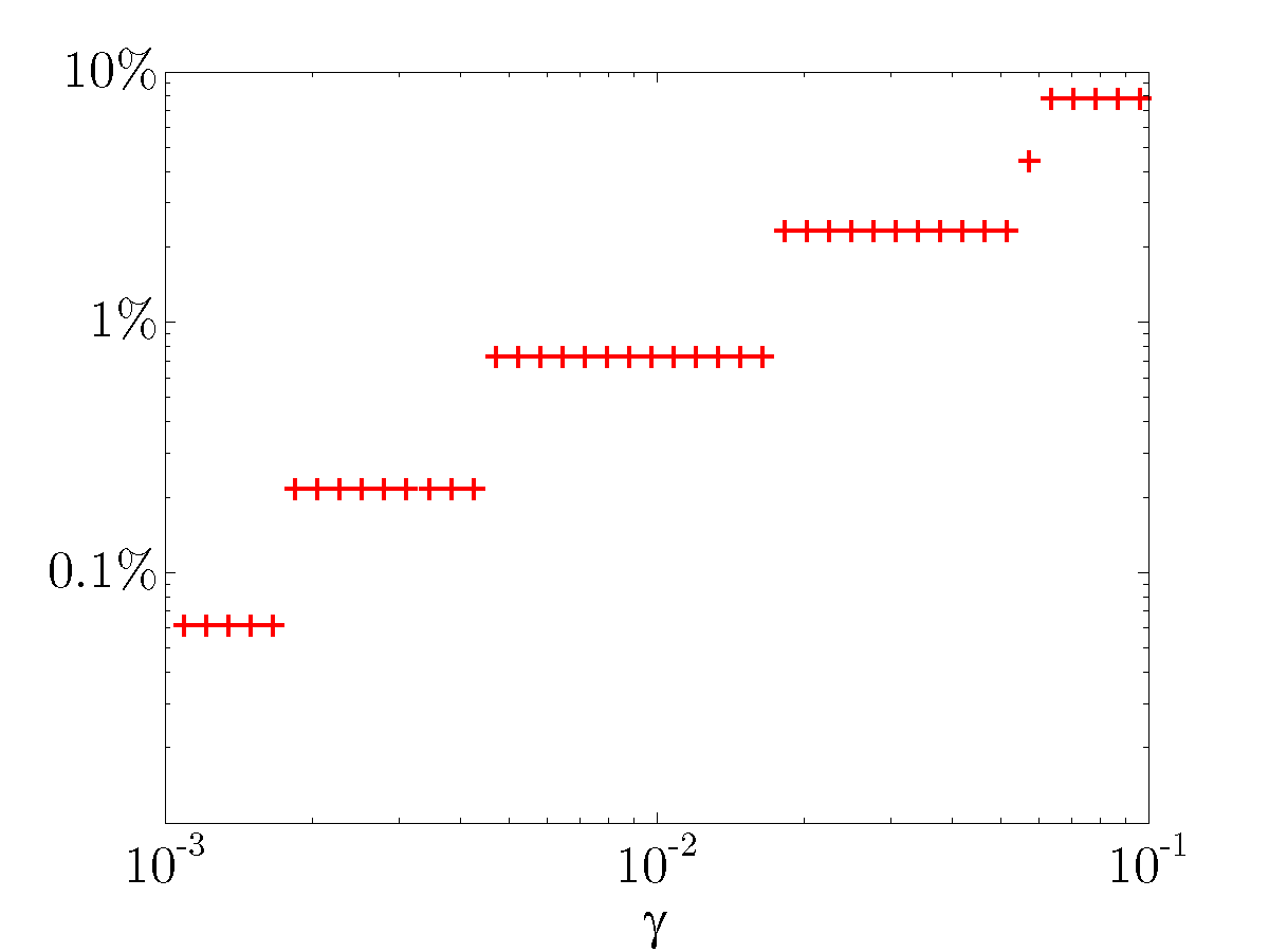 |
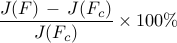
Performance loss:
|
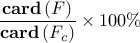
The above results demonstrate that the optimal sparse feedback gain,
with  of nonzero elements relative to the centralized feedback gain
  ,
introduces performance loss of only
,
introduces performance loss of only  compared to .
Sparsity vs. performance
![begin{array}{cccc} gamma & 0.014 & 0.043 & 0.10 [0.1cm] displaystyle{frac{ {rm bf{card}} , (F) }{ {rm bf{card}} , (F_{c}) }} & 9.36 % & 5.80 % & {bf 1.96} % [0.35cm] displaystyle{ frac{J(F) ,-, J(F_c)}{J(F_c)} } & 0.80 % & 2.31 % & {bf 7.80} % end{array}](eqs/3600077326593397941-130.png)
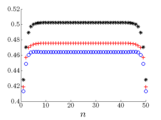
Diagonals of sparse feedback gains
The elements on the main diagonals of the optimal sparse feedback gains become larger as the number of
the sub-diagonals of drops. Thus, in order to compensate for communication with smaller
number of neighboring masses, each mass places more emphasis on its own position and velocity when
forming control action.
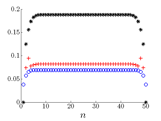 |
Diagonal of the optimal sparse |
 ,
,  ,
,  .
.
 |
Diagonal of the optimal sparse |
Also see computational results obtained using other sparsity-promoting functions.