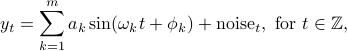
Separation of line spectra and system dynamics
Consider the following time-series
where  represents colored noise.
The routine L1AR.m estimates spectral lines together with an autoregressive (AR) component
corresponding to the noise. The routine and relevant theory are explained in [1] and rely on the ideas of compressive sensing (L1-optimization, sparse selection from a suitable dictionary). represents colored noise.
The routine L1AR.m estimates spectral lines together with an autoregressive (AR) component
corresponding to the noise. The routine and relevant theory are explained in [1] and rely on the ideas of compressive sensing (L1-optimization, sparse selection from a suitable dictionary).
helpL1ARhelp L1AR
  function [omega,mag,phi,a,sigma]=L1AR(y,freqNum,ARorder,freqrange,N)
  input
               y: observation record signal+noise
         freqNum: number of signals
         ARorder: order of autoregressive filter (default value 0)
       freqrange: interested frequency interval (default value [0 pi])
               N: resolution=2*pi/N (default value 2*length(y))
  output
           vopt:
          omega:  estimated frequencies of signals
            mag:  magnitudes of signals
            phi:  estimated phase angles
              a:  coefficients of AR filter
          sigma:  whitened noise variance
Needed software: convex optimization tool cvx.
Sample problem
Consider the following time-series
where  , ,  , , 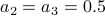 , ,  , ,  , ,  , ,  , ,  and and  . The resolution needed is . The resolution needed is  which is higher than Fourier analysis that is which is higher than Fourier analysis that is  .
The noise component is generated as the output of an AR filter having transfer function .
The noise component is generated as the output of an AR filter having transfer function
and driven by white noise with variance  .
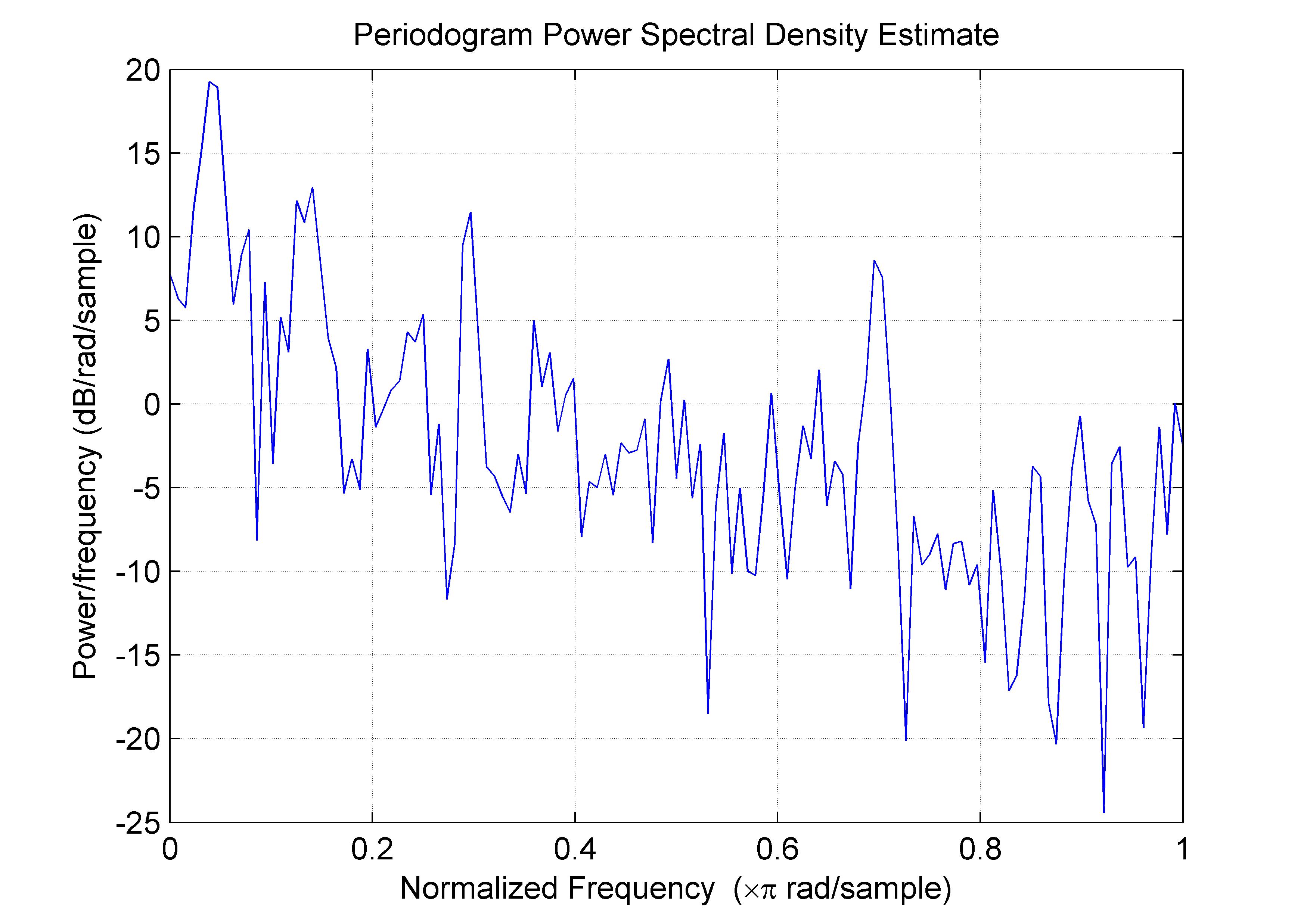
The periodogram of the observation record is shown in the following figure. .
The periodogram of the observation record is shown in the following figure.
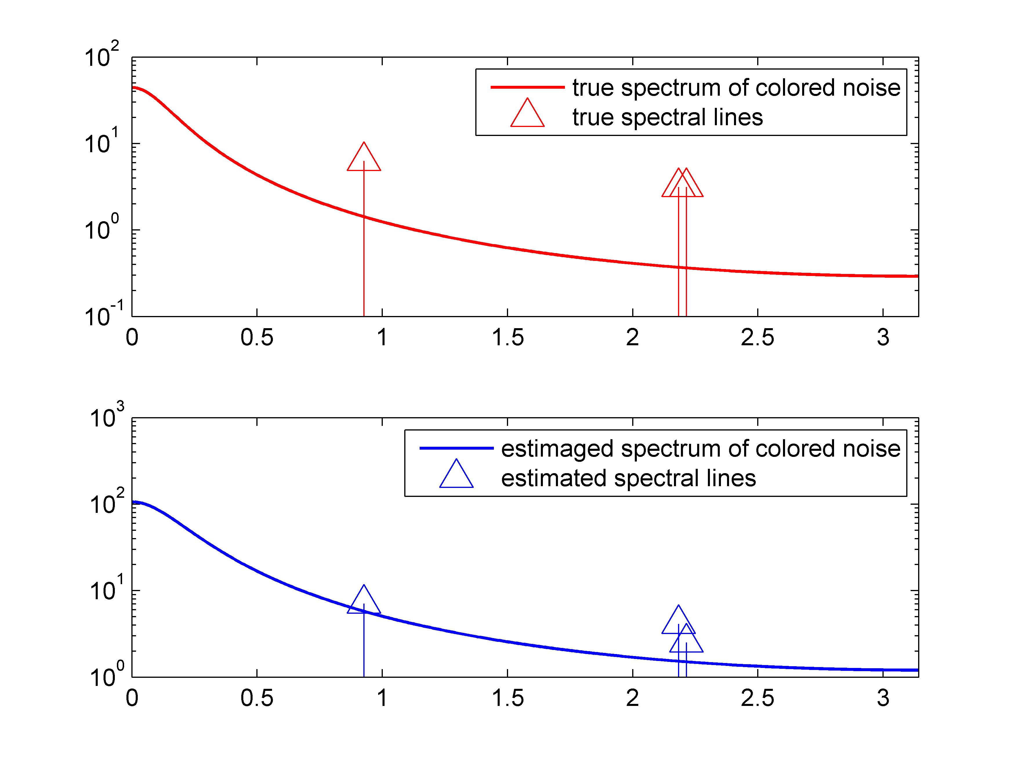
There are multiple peaks in the plot. The “ground truth” in the form of noise spectral density and spectral lines are shown in the first subplot of the following figure. The noise spectral density and
spectral lines which are approximated using L1AR.m are shown in the second subplot. All three frequencies are identified exactly at the chosen resolution scale. The code for this example is shown below.
testL1AR
o1 = 59*pi/200; phi1 = pi/4; a1 = 1;
o2 = 139*pi/200; phi2 = pi/3; a2 = .5;
o3 = 141*pi/200; phi3 = -pi/3; a3 = .5;
order = 1; sigma = 1.5;
a = [1.0000 -.85];
n = 150; t=0:n-1;
T = tf([1 zeros(1,order)],a,-1);
randn('seed',101); noise = sigma*randn(n,1);
sig = sin(o1*t+phi1)+.5*sin(o2*t+phi2)+.5*sin(o3*t+phi3);
y = lsim(T,noise)+sig';
freqNum = 3; N = 200;
[omega,mag,phi,a,sigma_est]=L1AR(y,freqNum,order,[0 pi],N);
w = linspace(0,pi,500);
ptrue = abs(freqresp(T,w)).^2;
T_est = tf([1 zeros(1,order)],a,-1);
pest = abs(freqresp(T_est,w)).^2*sigma_est^2;
figure(1); periodogram(y);
figure(2);
subplot(2,1,1);
plot(w,vec(ptrue),'r','LineWidth',1.2);hold on;
plot(o1,2*pi*a1,'r^','MarkerSize',12);
legend('true spectrum of colored noise','true spectral lines');
set(gca,'YScale','log','XLim',[0 pi]);
arrow([o1 o2 o3],(2*pi*[a1 a2 a3]),12);
subplot(2,1,2);
plot(w,vec(pest),'b','LineWidth',1.2);hold on;
plot(omega(1),2*pi*mag(1),'b^','MarkerSize',12);
legend('estimaged spectrum of colored noise','estimated spectral lines');
set(gca,'YScale','log','XLim',[0 pi]);
arrowb(omega,(2*pi*mag),12);
Reference
[1] L. Ning, T.T. Georgiou and A. Tannenbaum, “Separation of system dynamics and line spectra via sparse representation,” 49 th IEEE Conference on Decision and Control, 473-478, December 2010.
|