Distances and Riemannian metrics for multivariate spectral densities
 |
Preliminaries on multivariate prediction
Consider a multivariate discrete-time, zero mean, weakly stationary stochastic process 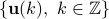 with
with  taking values in
  . Let
. Let

denote the sequence of matrix covariances and  be the corresponding matricial power spectral measure for which
We will be concerned with the case of non-deterministic process of full rank with an absolutely continuous power spectrum. Hence, 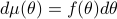 with
with  being a matrix valued power spectral density (PSD) function. Further,
  is assumed to be integrable throughout.
Geometry of multivariable process
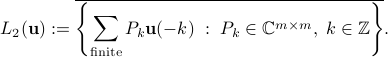
Define  to be the closure of
  -vector-valued finite linear combinations of
 with respect to convergence in the mean:
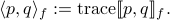
This space is endowed with both, a matricial inner product

as well as a scalar inner product

It is standard to establish the Kolmogorov isomorphism between the “temporal” space  and the “spectral” space
  ,
,
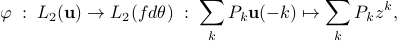
with  for
for ![thetain[-pi, pi]](eqs/1859324716-130.png) . It is convenient to endow the latter space the matricidal inner product
. It is convenient to endow the latter space the matricidal inner product
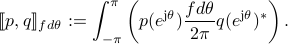
We denote 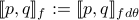 for simplicity. The corresponding scalar inner product
The least-variance linear prediction
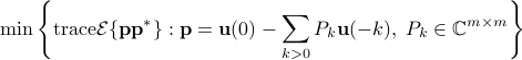
can be expressed in the spectral domain
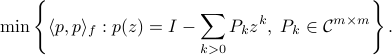
The minimizer coincides with that of

where the minimum is sought in the positive-definite sense. Let  denote the the minimizer of such a problem, then the minimal matrix of the above problem, denoted by
  , is
, is

Spectral factorization and optimal prediction
For a non-deterministic process of full rank, the determinant of the error variance is non-zero, and
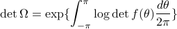
this the is well-known Szeg -Kolmogorov formula.
We consider only non-deterministic processes of full rank and hence we assume that
-Kolmogorov formula.
We consider only non-deterministic processes of full rank and hence we assume that
![log det f(theta)in L_1[-pi, pi].](eqs/1951284714-130.png) admits a unique factorization
admits a unique factorization
with  and
and  ,
where
,
where  , and
, and  denotes the Hardy space of functions which are analytic in the unit disk
  with square-integrable radial limits. The spectral factorization presents an expression of
the optimal prediction error in the form
with square-integrable radial limits. The spectral factorization presents an expression of
the optimal prediction error in the form
Comparison of PSD's
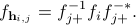
Prediction errors and innovations processes
Consider two processes  with
with  and
and  the corresponding PSD's and the optimal prediction filters, respectively.
Let
the corresponding PSD's and the optimal prediction filters, respectively.
Let

for  be an innovations process. Then, from stationarity,
whereas

The color of innovations and PSD mismatch
We normalize the innovation processes as follows:
then the power spectral density of the process  is
is
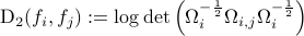
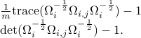
The mismatch between the two power spectra ,  can be quantified by the distance of
  to the identity. To this end, we define
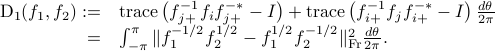
The following choices of divergence measures lead to the same Riemannian structure as the above one:
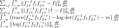
These are the Frobenius distance, the generalized Hellinger distance, the multivariate Itakuta-Saito distance, the log-spectral deviation between  and
and  , respectively.
Suboptimal prediction and PSD mismatch
As was given in  ,
,  .
The above equality holds if and only if
.
The above equality holds if and only if  . Thus a mismatch between the two spectral densities can be quantified by the strength of the above inequality. Since
 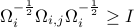 , we consider
as a “divergence measure” between the two PSD's. The following options lead to the same Riemannian structure:
Riemannian structure on multivariate spectra
Consider the following class of  PSD's
PSD's
![mathcal{F}:= {f | f(theta)>0, forall thetain[-pi, pi], df(theta)/dtheta mbox{~continuous} }.](eqs/1737006493-130.png)
Let  be a class of admissible perturbations of
  for
for  with
with

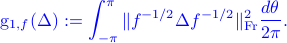
It was shown in [1] that for PSD's in  and in the distance
  induces the following Riemannian metric
In particular, for  and
and  . Then for
  sufficiently small

The geodesic path connecting two spectra  is
is

The geodesic distance is
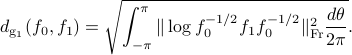
For the distance  , the corresponding Riemannian metic is

The associtated geodesic path for  is still unknown.
Examples
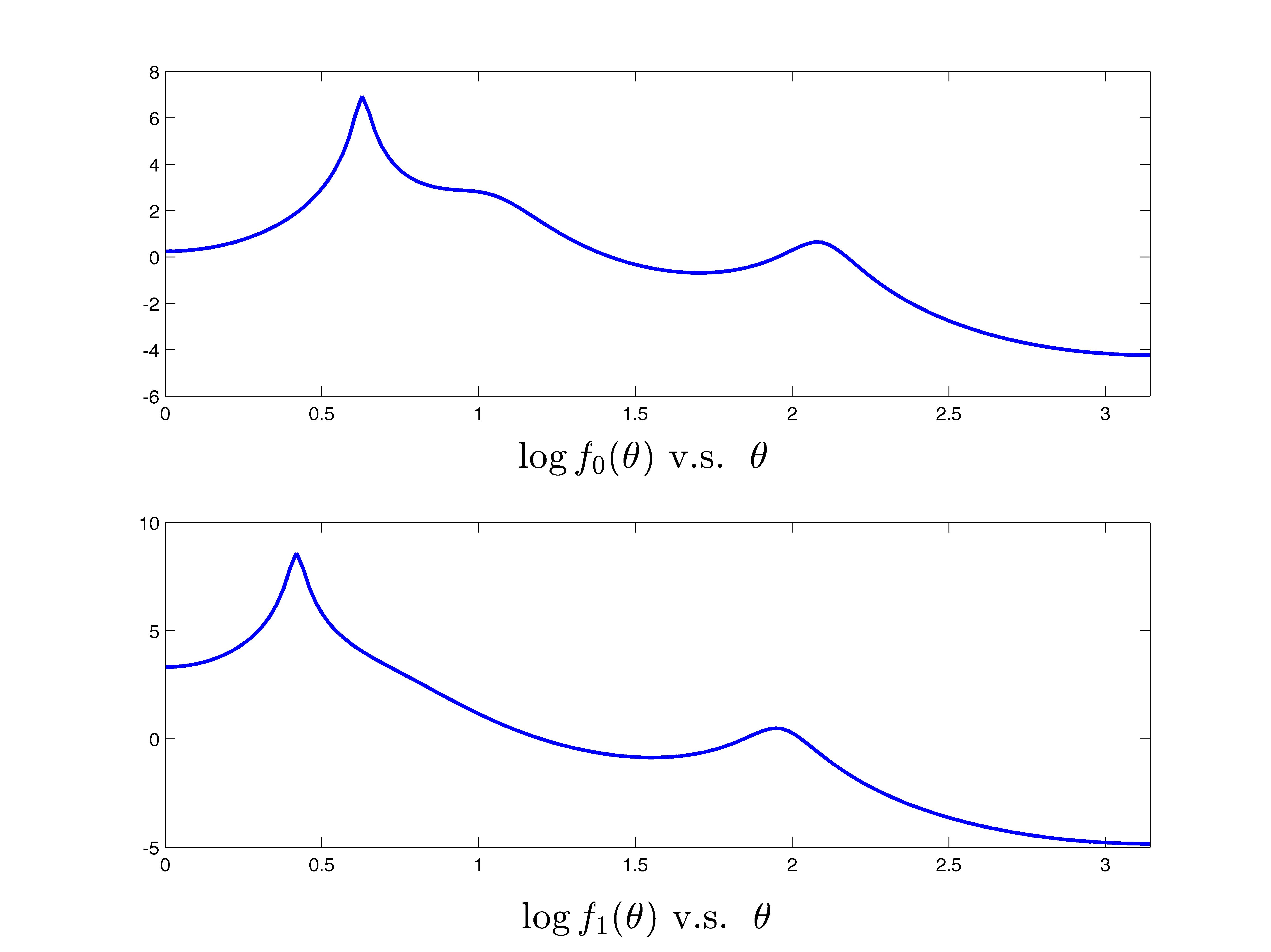
A scalar example
Consider the two power spectral densities
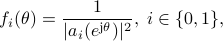
where

The two power spectra,  and
and  , are shown in the following figure.
 |
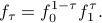
We evaluate 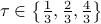 , the corresponding spectra are shown in the following figure.
 |
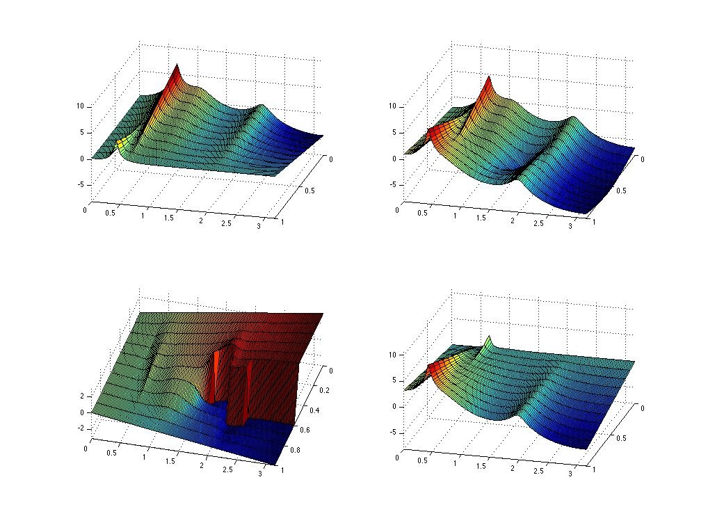
A multivariable example
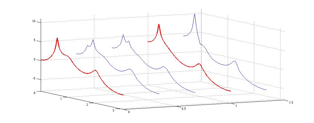
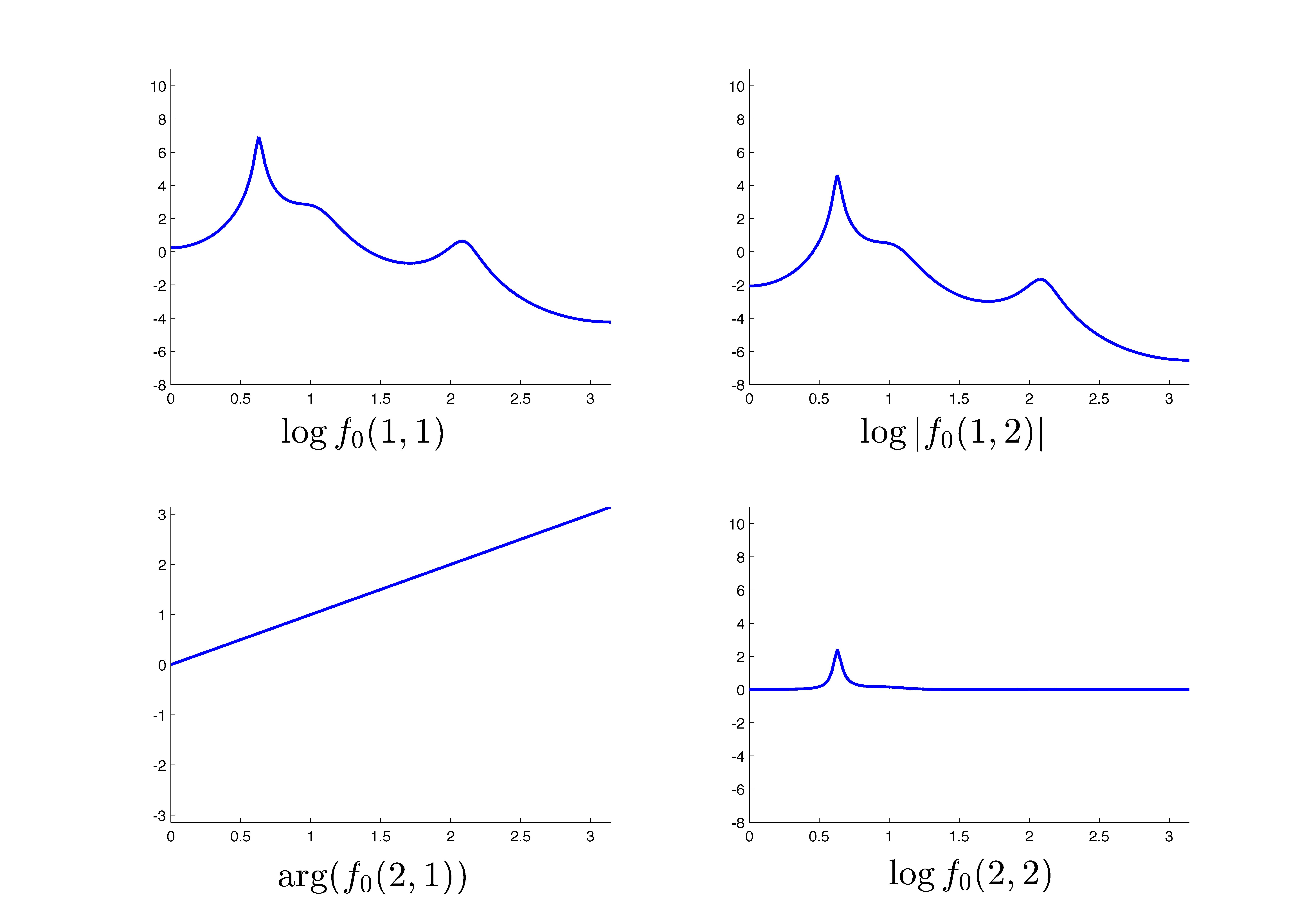
Consider the two matrix-valued power spectral densities
![f_0=left[ begin{array}{cc} 1 & 0 0.1e^{{rm j}theta} & 1 end{array} right]left[ begin{array}{cc} frac{1}{|a_0(e^{{rm j}theta})|^2} & 0 0 & 1 end{array} right]left[ begin{array}{cc} 1 & 0.1e^{-{rm j}theta} 0 & 1 end{array} right]](eqs/1234454410-130.png)
![f_1=left[ begin{array}{cc} 1 & 0.1e^{{rm j}theta} 0 & 1 end{array} right]left[ begin{array}{cc} 1 & 0 0 & frac{1}{|a_1(e^{{rm j}theta})|^2} end{array} right]left[ begin{array}{cc} 1 & 0 0.1e^{-{rm j}theta} & 1 end{array} right].](eqs/1825561106-130.png)
The following two figures show the two spectra where the  block is the
  and the
  block is
  , for
, for  .
.
 |
 |
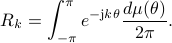
We compute the geodesic connecting  and
and  as
as

The geodesic is shown in the following figure.
|
|
Reference
[1] X. Jiang, L. Ning and T.T. Georgiou, “Distances and Riemannian metrics for multivariate spectral densities,” IEEE Trans. on Signal Processing, to appear 2012. http://arxiv.org/abs/1107.1345