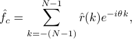
%  SIGNAL = sinusoids + noise
%  Setting up the signal parameters and time history
    N=100;
    a0=1.8; a1=1.5; theta1=1.3; a2=2; theta2=1.35;
    k=1:N; k=k(:);
    y=a0*randn(N,1)+a1*exp(1i*(theta1*k+2*pi*rand))+a2*exp(1i*(theta2*k+2*pi*rand));
High resolution tools for spectral analysis
Research supported by AFSOR, NSF. Maintained by L. Ning and T.T. Georgiou
 |
Introduction
Consider a discrete-time zero-mean stationary process  ,
,
 , and
let
, and
let
represents power density over frequency. Under suitable smoothness conditions, it is also
Spectral estimation refers to esimating  when only
a finite-sized observation record
when only
a finite-sized observation record  of the time series is available.
Different schools of thought have evolved over the years based on varying assumptions and formalisms. Classical methods began first
based on Fourier transform techniques and the periodogram, followed by the so called modern spectral estimation methods
such as the Burg method, MUSIC, ESPRIT, etc. The mathematics relates to the theory of the Szeg
of the time series is available.
Different schools of thought have evolved over the years based on varying assumptions and formalisms. Classical methods began first
based on Fourier transform techniques and the periodogram, followed by the so called modern spectral estimation methods
such as the Burg method, MUSIC, ESPRIT, etc. The mathematics relates to the theory of the Szeg orthogonal polynomials and the structure of Toeplitz covariances.
In contrast, recently, the analysis of state covariance matrices, see e.g. [1, 2], suggested a general framework which allows even higher resolution. A series of generalized spectral estimation tools have been developed generalizing Burg, Capon, MUSIC, ESPRIT, etc.. In the following, we will overview some of these high resolution methods and the relevant computer software. Their use is shown via a representative academic examples.
We want to resolve two sinusoids in based on  noisy measurements of the time series

where  and
and  . These are closer than
the theoretical resolution limit
. These are closer than
the theoretical resolution limit  of Fourier method.
FFT-based methods
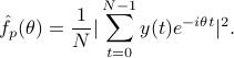
We begin with two classical formulae. The correlogram is defined as
where  denotes an estimate of the covariance lag
  , whereas the periodogram
The two coincide when the correlation lag is estimated via

where 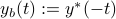 . The periodogram can be efficiently computed using the fast Fourier transform (FFT).
There is a variety of methods, such as Welch and Blackman-Tukey methods, designed to improve the performance using lag window functions either in the time domain or in the correlation domain.
In situations when the data length is short, to get a smooth spectrum, we may
increase the data length
by padding zeros to the sequence.
. The periodogram can be efficiently computed using the fast Fourier transform (FFT).
There is a variety of methods, such as Welch and Blackman-Tukey methods, designed to improve the performance using lag window functions either in the time domain or in the correlation domain.
In situations when the data length is short, to get a smooth spectrum, we may
increase the data length
by padding zeros to the sequence.
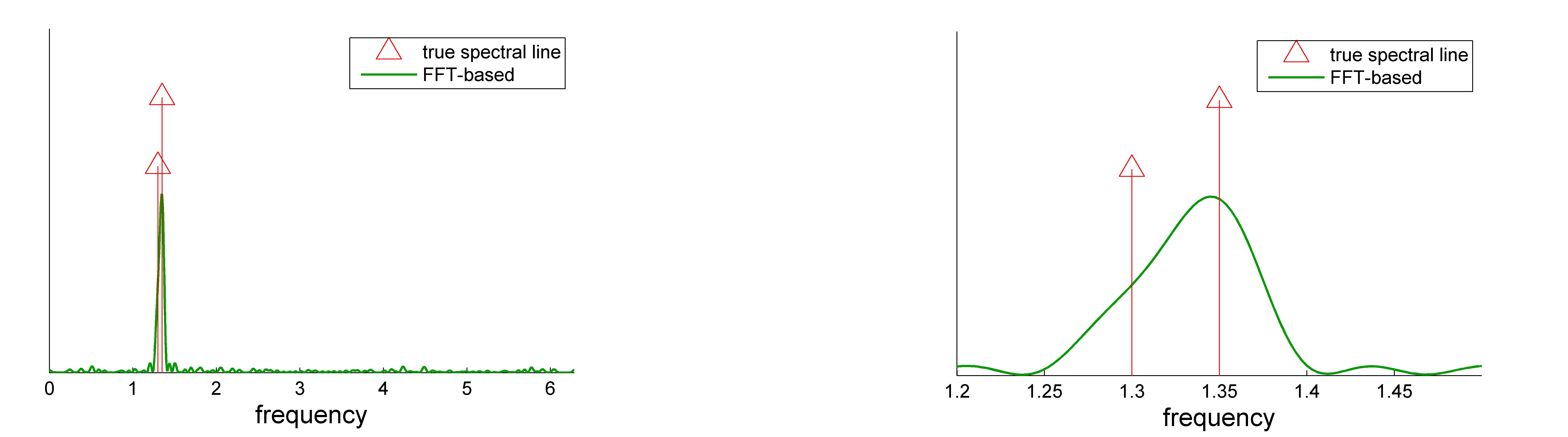
Using the above example, we pad up  by adding zeros. The corresponding
FFT-based spectrum is shown in the following figures.
Rudimentary code is displayed as a demonstration. A file to reproduce the following results can
be downloaded. Alternative matlab build-in routines for periodograms are periodogram, pwelch, etc.
by adding zeros. The corresponding
FFT-based spectrum is shown in the following figures.
Rudimentary code is displayed as a demonstration. A file to reproduce the following results can
be downloaded. Alternative matlab build-in routines for periodograms are periodogram, pwelch, etc.
% the fft-based spectra
NN=2048; th=linspace(0,2*pi,NN);
Y =abs(fft(y,NN))/sqrt(N);
Y = Y.^2;
plot(th,Y);
 |
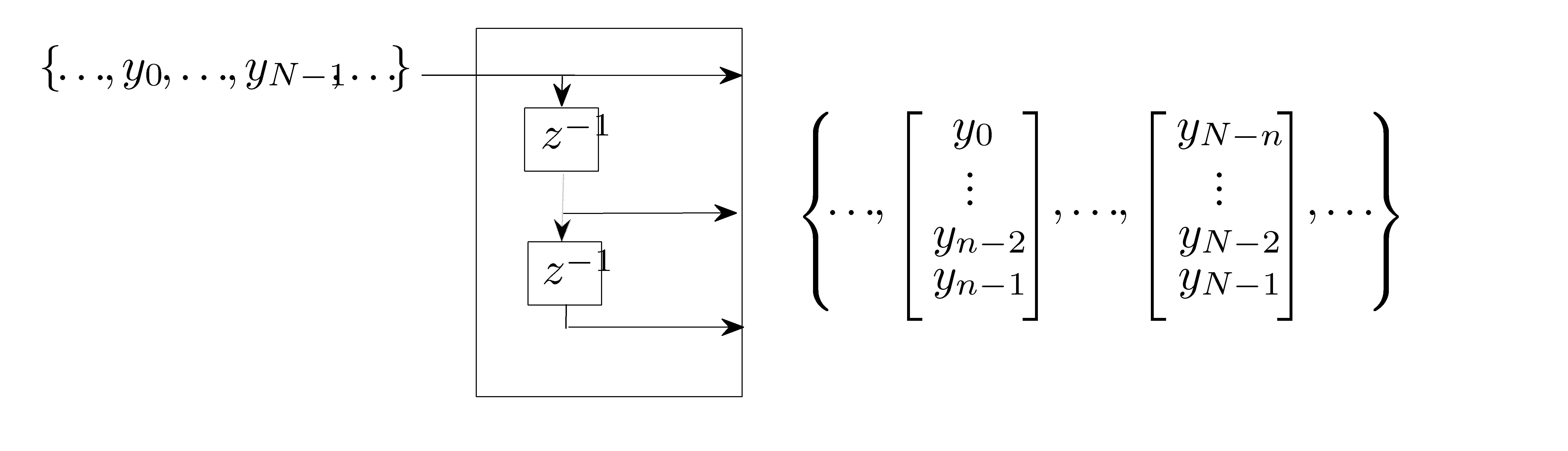
Input-to-state filter and state covariance
The first step to explain the high resolution spectral analysis tools is to consider the input-to-state
filter below and the corresponding
the state statistics.
The process  is the input and
  is the state.
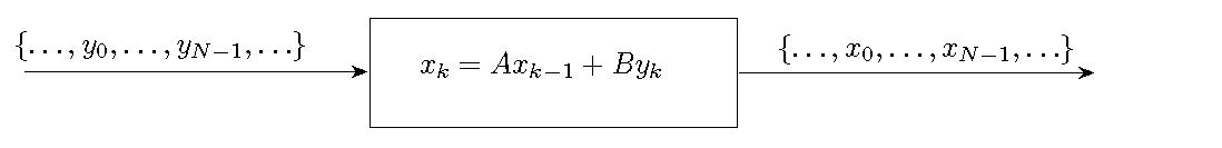 |
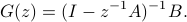
Then the filter transfer function is
A positive semi-definite matrix  is the state covariance of the above filter, i.e.
 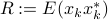 for some stationary input
process
for some stationary input
process  , if and only if it satisfies the following
equation
, if and only if it satisfies the following
equation

for some row-vector  .
Starting from a finite number of samples, we denote
.
Starting from a finite number of samples, we denote
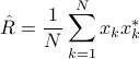
the sample state covariance matrix.
If the matrix  is the companion matrix
![A = left[ begin{array}{ccccc} 0 & 0 & ldots & 0 & 0 1 & 0 & ldots & 0 & 0 vdots & vdots & & vdots& vdots 0 & 0 & ldots & 1 & 0 end{array} right], ~~ B= left[ begin{array}{c} 1 0 vdots 0 end{array} right], hspace*{3cm} (1)](eqs/720422545-130.png)
the filter is a tapped delay line:
 |
The corresponding state covariance is Toeplitz matrix. Thus the state-covariance formalism subsumes the theory of Toeplitz matrices.
The input-to-state filter works as a “magnifying glass” or, as type of bandpass filter, amplifying the harmonics in a particular frequency interval.
Shaping of the filter is accomplished via selection of the eigenvalues of . In the above example, we set  eigenvalues of at
  , and the phase
angle
, and the phase
angle  is the middle of the interval
 ![[theta_1,;theta_2]](eqs/922774589-130.png) where resolution is desirable. Then we build the pair
where resolution is desirable. Then we build the pair  using routine cjordan.m, (and rjordan.m for real valued
problem).
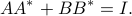
The pair is normalized to satisfy
using routine cjordan.m, (and rjordan.m for real valued
problem).
The pair is normalized to satisfy
The routine dlsim_complex.m generate the state covariance matrix (dlsim_real.m for
real valued problem).
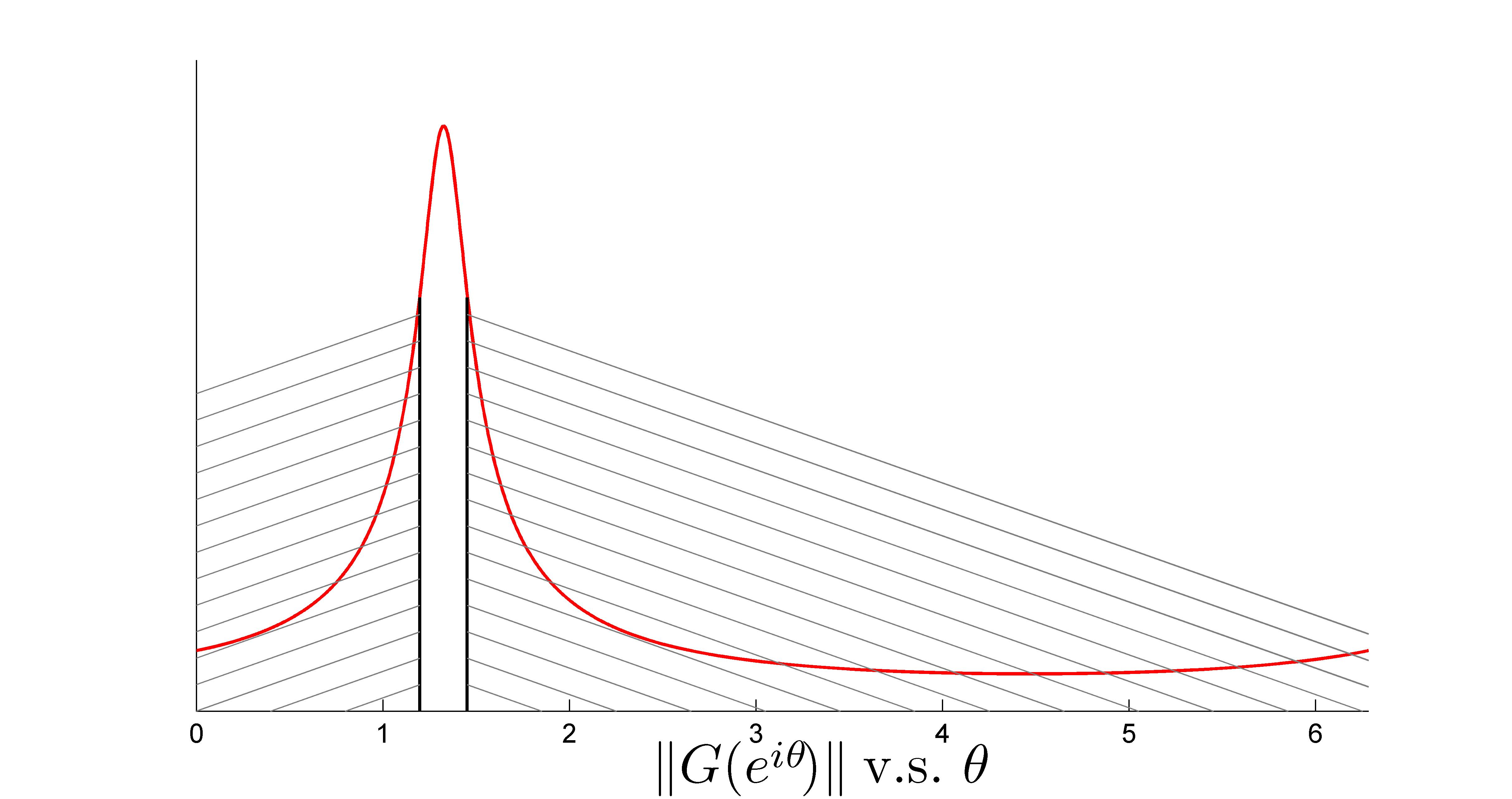
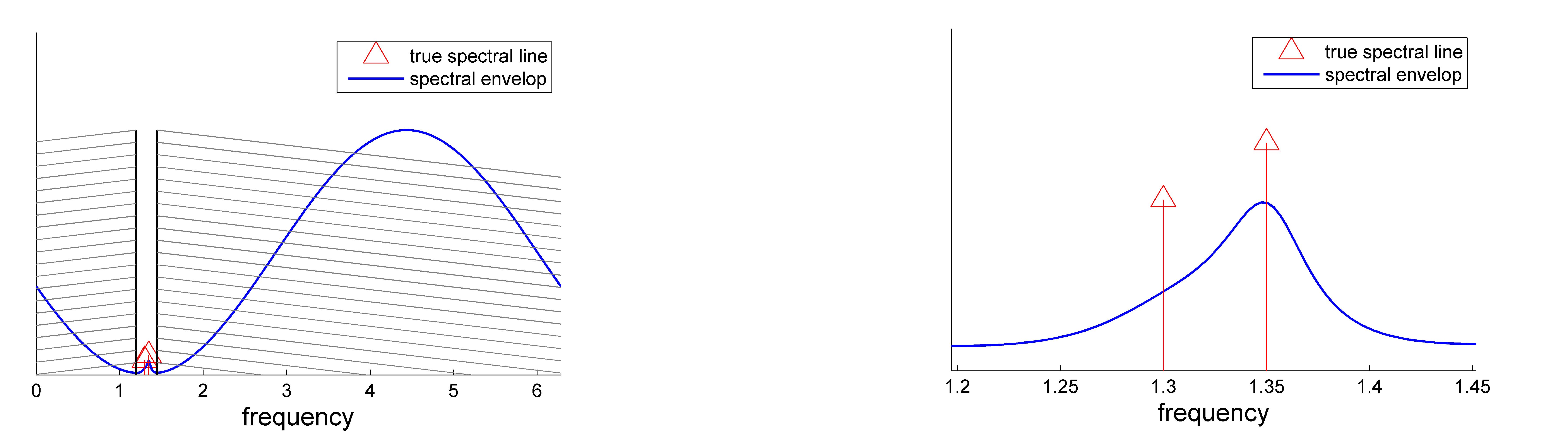
The following figure plots  versus
  . The gain
at equal
. The gain
at equal  and
and  is approximately
  dB below the peak value. The window is marked in the following figure. The figure to the right shows the detail within the window of interest.
% setting up filter parameters and the svd of the input-to-state response
thetamid=1.325;
[A,B]=cjordan(5,0.88*exp(thetamid*1i));
% obtaining state statistics
R=dlsim_complex(A,B,y');
sv=Rsigma(A,B,th);
plot(th(:),sv(:));
 |
Maximum entropy spectrum
The entropy of a probability distribution function  with
with  ,
,
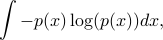
quantifies the uncertainty of the corresponding random variable.
When is a multi-dimensional Gaussian distribution with zero mean and covariance matrix
 , the entropy becomes
For a zero-mean stationary Gaussian process  , corresponding to
infinite-sized Toeplitz structured covariance, the entropy “diverges”. Thus, one uses instead the ‘‘entropy rate". Let
, corresponding to
infinite-sized Toeplitz structured covariance, the entropy “diverges”. Thus, one uses instead the ‘‘entropy rate". Let  be a
be a  dimensional principle sub-matrix of the
covariance matrix
dimensional principle sub-matrix of the
covariance matrix
![T_{N-1}=left[ begin{array}{cccc} r(0) & r(1) & ldots & r(N-1) r(-1) & r(0) & ldots & r(N-2) vdots & vdots & ddots & cdots r(-N+1) & r(-N+2) & r(-1) & r(0) end{array} right],](eqs/2065058937-130.png)
Then the entropy rate is

The limit of  converges to the optimal one-step prediction error variance, and from the Szeg
 -Kolmogorov formula
Given state statistics, the maximum entropy power spectrum is

The solution to this problem (see [2]) is

where
and  is the input-to-state filter defined above.
This formula subsumes the classical Burg method/AR modeling where the is a Toeplitz matrix and
is tapped delay line filter.
is the input-to-state filter defined above.
This formula subsumes the classical Burg method/AR modeling where the is a Toeplitz matrix and
is tapped delay line filter.
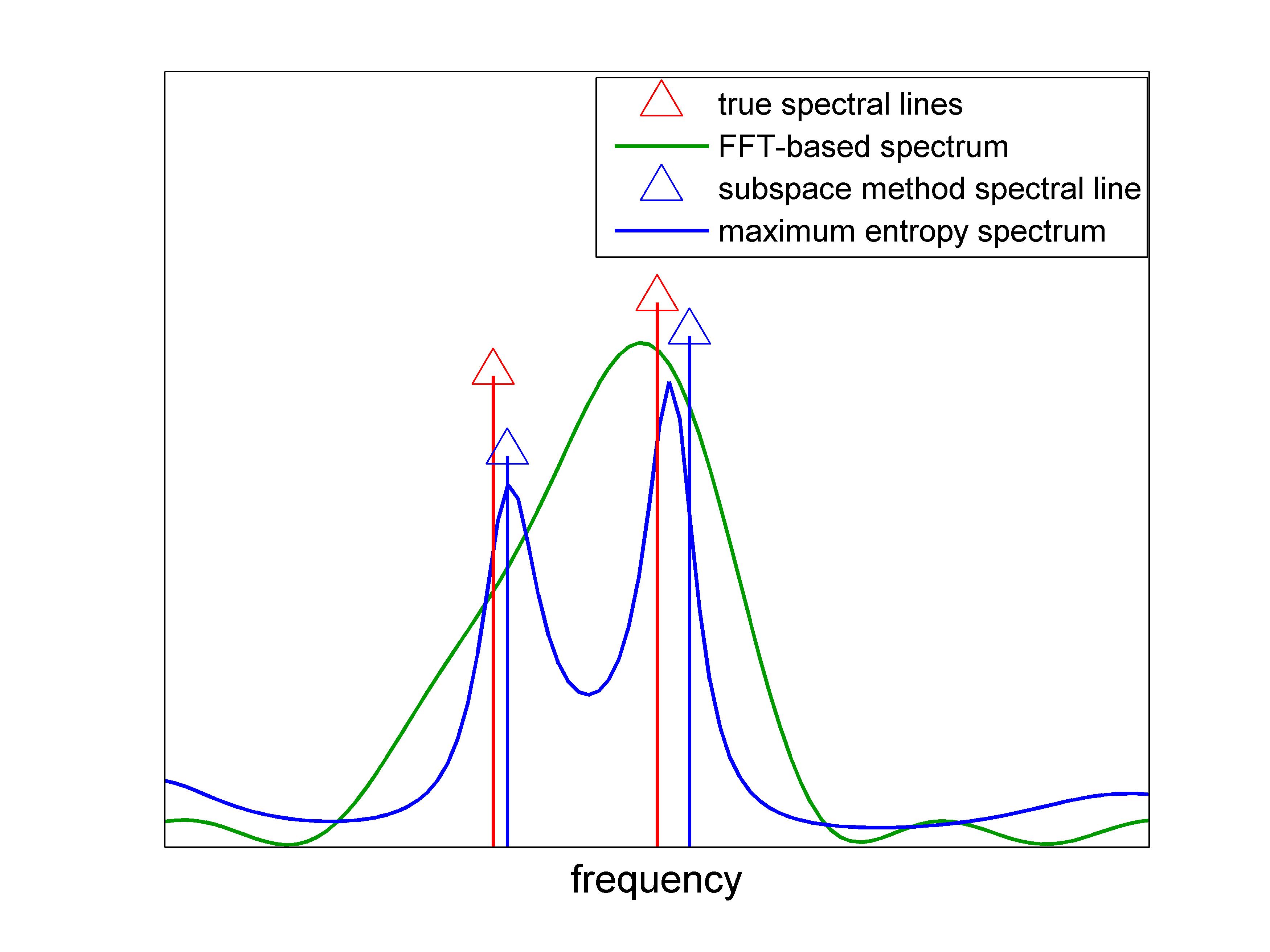
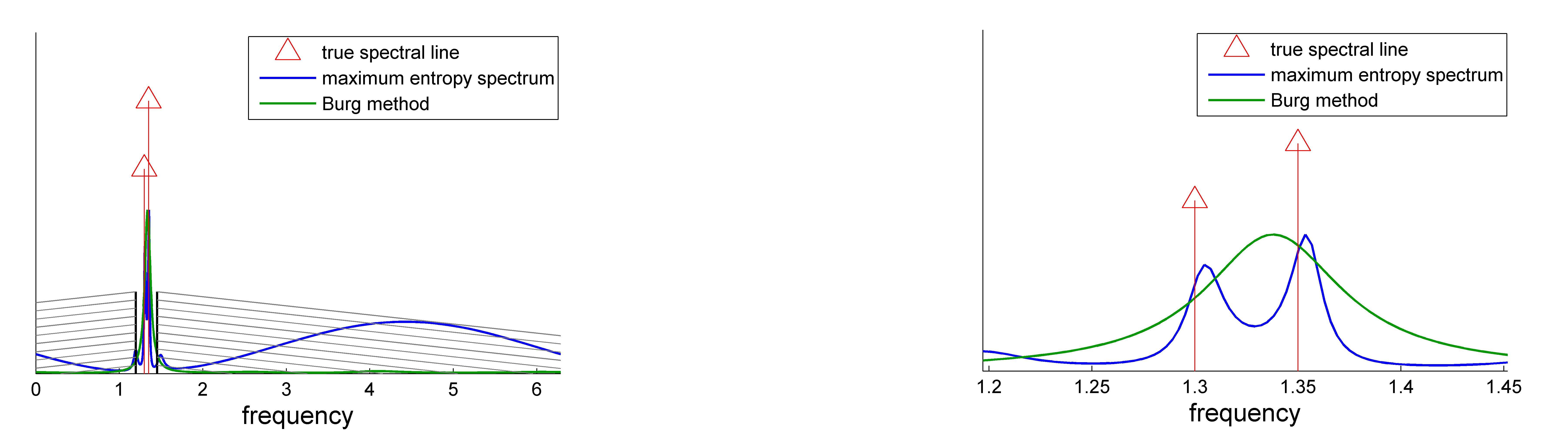
The maximum entropy spectrum is obtained using the routine me.m. For the example discussed above, the maximum entropy spectrum is shown in blue. There are two peaks detected inside the window. Burg's spectrum is shown in green. The resolution of Burg's solution is not sufficient to distinguish the two peaks.
% maximum entropy spectrum and Burg spectrum
me_spectrum=me(R,A,B,th);
plot(th,me_spectrum);
me_burg=pburg(y,5,th);
hold on;
plot(th,me_burg);
 |
Subspace methods
We start with the Carath odory-Fejr-Pisarenko result for Toeplitz matrices. Given a
  positive definite
Toeplitz matrix
positive definite
Toeplitz matrix  ,
let
,
let  be the smallest number such that
  is singular and has rank
  , then
has the formE
, then
has the formE
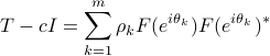
where
![F(e^{itheta_k})= left[ begin{array}{c} 1 e^{itheta_k} vdots e^{i(n-1)theta_k} end{array} right].](eqs/1272814962-130.png)
Accordingly, the power spectrum decomposes as
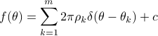
where  is the Dirac function. The decomposition corresponds to a set of white noise. See MA decomposition for a decomposition corresponds moving-average (MA) noise.
The above result can be generalized to the case of state covariances [1].
More specifically, let  be the unique solution to the Lyapunov equation
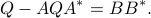
The matrix is the state covariance when the input is pure white noise. Let now be an arbitrary state covariance, let  be the smallest eigenvalues of the matrix pencil
  , and assume that the rank of
  is
is  , then
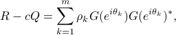
where  is generalization of
  .
.
The subspace spectral analysis methods rely on the singular value decomposition

where  is a unitary matrix and
  ,
,  . Partition
![U=[U_{1:m},; U_{m+1:n}]](eqs/272044314-130.png)
where  and
and  are the first and the last
  columns of , respectively.
Based on this decomposition, there are two ways we can proceed generalizing the MUSIC and ESPRIT methods, respectively [P. Stoica, R.L. Moses, 1997].
columns of , respectively.
Based on this decomposition, there are two ways we can proceed generalizing the MUSIC and ESPRIT methods, respectively [P. Stoica, R.L. Moses, 1997].
Noise subspace analysis
The columns of span the null space of  , while the signal
  ,
,  is in the span of the columns of .
So the nonnegative trigonometric polynomial
is in the span of the columns of .
So the nonnegative trigonometric polynomial

has roots at  .
.
Given a sample state covariance matrix  and an estimate on the number of signals , we let
  be the matrix of singular vectors of the smallest singular values, and
  be
the corresponding trigonometric polynomial for . Two possible generalization of the MUSIC method are as follows.
be
the corresponding trigonometric polynomial for . Two possible generalization of the MUSIC method are as follows.
Spectral MUSIC: identify
 , for as the values on
 ![[-pi,; pi]](eqs/481304345-130.png) where
where
 achieves the -highest local maxima.
Root MUSIC: identify
, for as the angle of the -roots of  which have amplitude
  and are closest to unit circle.
Signal subspace analysis
A signal subspace method relies on the fact that for the pair ,  and given above, there is a unique solution to the following matrix equation
![U_{1:m} =[B ~ AU_{1:m}] left[begin{array}{c}muPhi end{array} right],](eqs/1198537117-130.png)
where  is
is  row vector and
  a
a  matrix. The eigenvalues of are
precisely
matrix. The eigenvalues of are
precisely  for .
If is a Toeplitz matrix and , given as in
for .
If is a Toeplitz matrix and , given as in  with a companion matrix, then we
recover the ESPRIT result [P. Stoica, R.L. Moses, 1997].
with a companion matrix, then we
recover the ESPRIT result [P. Stoica, R.L. Moses, 1997].
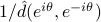
The signal subspace estimation is computed using sm.m, whereas music.m and esprit.m implement the MUSIC and ESPRIT methods, respectively. For the example discussed above, the estimated spectral lines are shown in the following figure. For an extensive comparison of the high resolution method sm.m with MUSIC and ESPRIT methods, see the example.
% subspace method
[thetas,residues]=sm(R,A,B,2);
arrowb(thetas,residues); hold on;
Ac=compan(eye(1,6));
Bc=eye(5,1);
That=dlsim_complex(Ac,Bc,y');
[th_esprit,r_esprit]=sm(That,Ac,Bc,2); % ESPRIT spectral lines
arrowg(th_esprit,r_esprit);
 |
Spectral envelop
Let  denote a spectral measure of the stochastic process
  , the envelop of maximal spectral power is defined as

where represents the state covariance and is the input-to-state filter. In other words,  represents the maximal spectral “mass” located at which is consistent with the covariance matrix. It can also be shown that

where  represents the state covariance for the sinusoidal input
  .
The optimal solution is
.
The optimal solution is
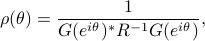
and implemented in envlp.m.
This generalizes the Capon spectral estimation method which applies to being Toeplitz matrix and the tapped delay line transfer function. The Capon method may be motivated by a noise suppression formulation aimed at antenna array applications [P. Stoica, R.L. Moses, 1997].
For real valued processes with a symmetric spectrum with respect to the origin, a symmetrized version of the spectral envelop [1] can be similarly obtained:

% spectral envelop
rhohalf = envlp(R,A,B,th);
rho = rhohalf.^2;
plot(th,rho);
 |
Reference
[1] T.T. Georgiou, “Spectral Estimation via Selective Harmonic Amplification,” IEEE Trans. on Automatic Control, 46(1): 29-42, January 2001. [BIBTEX]
[2] T.T. Georgiou, “Spectral analysis based on the state covariance: the maximum entropy spectrum and linear fractional parameterization,” IEEE Trans. on Automatic Control, 47(11): 1811-1823, November 2002. [BIBTEX]