Subspace methods

We start with the Carathodory-Fejr-Pisarenko result for Toeplitz matrices. Given a ntimes n positive definite Toeplitz matrix , let c>0 be the smallest number such that T-cI is singular and has rank m<n , then T-cI has the formE

$T-cI=sum_{k=1}^m rho_k F(e^{itheta_k})F(e^{itheta_k})^*$

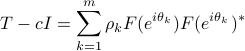
where

$F(e^{itheta_k})= left[ begin{array}{c} 1 e^{itheta_k} vdots e^{i(n-1)theta_k} end{array} right].$

Accordingly, the power spectrum f(theta) deomposes as

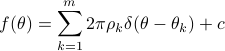
$f(theta)= sum_{k=1}^m 2pirho_k delta(theta-theta_k)+c$

where delta(cdot) is the Dirac function. The decomposition corresponds to a set of white noise. See MA decomposition for a decomposition corresponds moving-average (MA) noise.

The above result can be generalized to the case of state covariances [1]. More specifically, let be the unique solution to the Lyapunov equation

The matrix is the state covariance when the input is pure white noise. Let now be an arbitray state covariance, let be the smallest eigenvalues of the matrix pencil R-rho Q , and assme that the rank of R-c Q is , then

$R-c Q=sum_{k=1}^m rho_k G(e^{itheta_k}) G(e^{itheta_k})^*,$

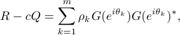
where $G(e^{itheta})$ is generalization of $F(e^{itheta})$ .

The subspace spectral analysis methods rely on the singular value decomposition

$R-cQ= U mbox{diag}{lambda_1, lambda_2, ldots, lambda_m, 0,ldots, 0 } U^*,$

where is a unitary matrix and lambda_k>0 , k=1,ldots, m . Partition

$U=[U_{1:m},; U_{m+1:n}]$

where $U_{1:m}$ and $U_{m+1:n}$ are the first and the last n-m columns of , respectively. Based on this decomposition, there are two ways we can proceed generalizing the MUSIC and ESPRIT methods, respectively [P. Stoica, R.L. Moses, 1997].

Noise subspace analysis

The columns of $U_{m+1:n}$ span the null space of R-cQ , while the signal $G(e^{itheta_k})$ , k=1,ldots, m is in the span of the columns of $U_{1:m}$ . So the nonnegative trigonometric polynomial

$d(e^{itheta},e^{-itheta})=G(e^{itheta})^* U_{m+1:n}U_{m+1:n}^*G(e^{itheta})$

has roots at ${theta_1, ldots, theta_m }$ .

Given a sample state covariance matrix hat{R} and an estimate on the number of signals m<n , we let $hat{U}_{m+1:n}$ be the matrix of singular vectors of the smallest singular values, and $hat{d}(e^{itheta},e^{-itheta})$ be the corresponding trigonometric polynomial for $hat{U}_{m+1:n}$ . Two possible generalization of the MUSIC method are as follows.

Spectral MUSIC: identify , for as the values on where $1/hat{d}(e^{itheta},e^{-itheta})$ achieves the -highest local maxima.
Root MUSIC: identify , for as the angle of the -roots of $hat{d}(z, z^{-1})$ which have amplitude and are closest to unit circle.

Signal subspace analysis

A signal subspace method relies on the fact that for the pair , and $U_{1:m}$ given above, there is a unique solution to the following matrix equation

$U_{1:m} =[B ~ AU_{1:m}] left[begin{array}{c}muPhi end{array} right],$

where is 1times m row vector and Phi a mtimes m matrix. The eigenvalues of Phi are precisely $e^{itheta_k}$ for k=1,ldots, m . If is a Toeplitz matrix and , given as in (1) with a companion matrix, then we recover the ESPRIT result [P. Stoica, R.L. Moses, 1997].

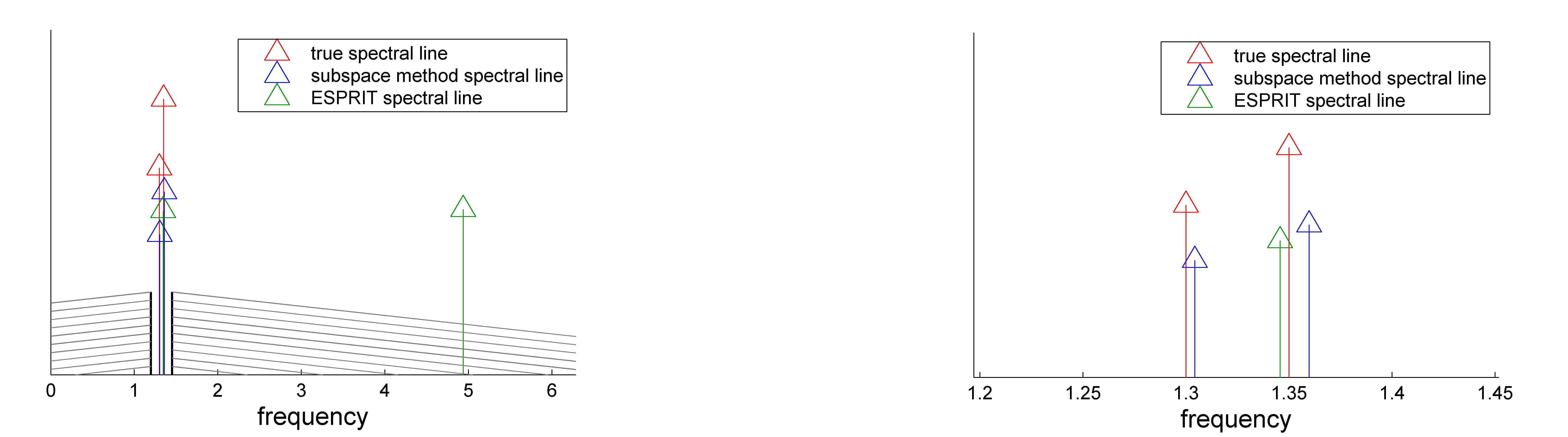
The signal subspace estimation computed using sm.m, whereas music.m and esprit.m implement the MUSIC and ESPRIT methods, respectively. For the example discussed above, the estimated spectral lines are shown in the following figure. For an extensive comparison of the high resolution method sm.m with MUSIC and ESPRIT methods, see the example.

smspectrum

% subspace method
[thetas,residues]=sm(R,A,B,2);
arrowb(thetas,residues); hold on;
Ac=compan(eye(1,6));
Bc=eye(5,1);
That=dlsim_complex(Ac,Bc,y'); 
[th_esprit,r_esprit]=sm(That,Ac,Bc,2); % ESPRIT spectral lines
arrowg(th_esprit,r_esprit);